Steel Column Design using Eurocode 3 - A Complete Guide
![[object Object]](/_next/image?url=%2Fimages%2Fauthors%2Fcallum_wilson.jpg&w=256&q=75)
Welcome to this, the second part in our series exploring structural steel design to Eurocode 3. The tutorial is focussed on steel column design.
In the previous tutorial on steel beam design, we introduced the Eurocode 3 document and in particular, Eurocode 3 Part 1-1: General rules and rules for buildings. We won't repeat this here, so refer back to part 1 now if you haven’t read it yet.
This is another quite long and detailed tutorial, so again, my advice is to tackle it in multiple sittings! It’s broken up as follows:
✅ Section 1: Eurocode 3 and Compression Members
In this first section, we’ll discuss how Eurocode 3 classifies compression members based on the actions that they must resist. This is critical as different classifications attract different design checks.
✅ Section 2: Steel Column Design Workflow
In section 2 we explore the column design workflow, using our what, where, why, how model. We’ll explain each step in the design workflow making sure to spend time understanding the motivations behind each design check as well as where in the code the design check is specified. This is quite a lengthy and detailed section but it will serve as a helpful reference, particularly as we move onto our worked example in the next section.
✅ Section 3: Steel Column Design - Worked Example
In this section, we work through a complete column design example. The design example has been constructed to attract as many of the design checks as possible in order to demonstrate the full breadth of the design process.
Essentially, we’ll be tackling a complex bi-axial bending design scenario. Once you’ve completed this example, 90% of practical column designs will look quick and easy by comparison!
✅ Section 4: Initial Sizing of Steel Columns
Luckily not all column designs are as involved as the example we considered in the previous section. So, it will be helpful to understand how the process is simplified for more straightforward design scenarios. We’ll cover this in section 4, giving you a more commonly used design flow for more typical column designs.
✅ Section 5: Wrapping up and Coming up next
In the final section, we briefly reflect on what we’ve achieved and briefly tee-up the next instalment of this steel design tutorial series!
1.0 Eurocode 3 and Compression Members
As we know, Eurocode 3 categorises design checks based on the internal forces developed in the member. Steel members which primarily resist axial compression are called columns. They represent one of the major structural components used across the world.
One of the most important ideas to grasp when considering the design of columns to Eurocode 3 is that although columns do predominantly resist axial compression, they may also resist bending moments - to a greater or lesser extent, depending on their configuration within the wider structure.
Eurocode 3 sets out a series of design checks which validate both the cross-sectional resistance and buckling resistance of compression members. In this sense, the design of columns and beams to Eurocode 3 is a similar process.
As is true for most Eurocode designs, we consider both the ultimate limit state (ULS) and serviceability limit states (SLS). However, for columns, we are almost exclusively concerned with the ULS case. Why is this? By the end of the article, you will be able to answer this question!
A steel column is one type of compression member. Other types of compression members do exist, for example, struts within braced frames or the top chord of a sagging truss. This article will only cover the design of steel columns but the majority of the design checks can be applied to other, more general forms of compression member.
1.1 Types of Column
Recall that we reached the conclusion that steel columns are a form of compression member which predominantly resists axial compressive forces. Prior to undertaking any Eurocode 3 design work, it’s critical that we recognise three distinct types of column behaviour. Recognising which behaviour our column most closely represents will be extremely useful when it comes to completing a Eurocode 3-compliant design.
Note that this article is concerned with the design of structural steel columns. We will not discuss the theoretical background to column buckling. This is discussed in our column buckling series (part 1, part 2 and part 3).
1.1.1 Simple columns
As the name would suggest, simple columns represent the simplest form of column behaviour. So what makes a column simple?
In fact a simple column is any column which forms part of a simple structure. A simple structure is composed of members connected by pinned joints and which resists horizontal loads by way of bracing elements rather than via frame action.
The definition of a simple column is as follows…
'a simple column is a compression member which is designed for the prevailing and predominant axial force but also for a nominal bending moment which is induced in the column due to the eccentricity of the transferred force between beam and column at connection points.'
Importantly, the eccentricity, , of the vertical load is typically no larger than and therefore the design bending moment acting upon the column is typically not large.
1.1.2 Uniaxial beam-columns
Simple structures are extremely popular in modern construction as they permit efficient design and fast construction. In many cases, bracing elements can provide horizontal stability, making simple construction a much-favoured choice.
However, there are structures where bracing elements are not suitable. For example, consider a typical portal-framed structure. When lateral loads are applied in the plane of the portal frames, bending moments that develop at the column-rafter connections are the mechanism by which lateral stability is achieved. Bracing is typically provided to resist lateral loads which act out of plane. We discuss lateral stability further in this tutorial.
From this observation, we can deduce that in response to in-plane loading, the portal columns will experience axial force and uniaxial bending i.e. bending about an axis perpendicular to the span of the rafters (typically the major principal axis for the column section).
This leads us to the notion of a 'beam-column'. There is no set magnitude of bending moment at which a simple column becomes a beam-column; this is left to the Engineer's judgment.
Put simply, if your column is experiencing significant bending moments about a single axis in addition to axial force, then it should be classified as a uniaxial beam-column.
1.1.3 Biaxial beam-columns
As you might have guessed, a biaxial beam-column is a further progression from the uniaxial beam-column. A biaxial beam-column experiences axial force and significant bending moments about both of its principal axes.
Remember: for both the uniaxial and biaxial beam-column cases, a suitable connection must be detailed between beam and column which permits the transfer of bending moments between these elements. We won’t be covering connection design in this tutorial.
Initially, it can be confusing to categorise a column into one of the above three categories. This tutorial will provide you with all of the tools needed to assess each type of column. Fortunately, if you wrongly classify a simple column as a bi-axial beam-column, the design checks will actually result in a more efficient design than if you had jumped straight into the simplifications afforded by a classification as a simple column.
2.0 Steel Column Design Workflow
The following section will identify and explain the design steps which are necessary for steel column design to Eurocode 3. Just like in the previous steel beam design tutorial, the purpose of this section is to highlight
- what the checks are,
- how to conduct the checks
- and most importantly, why we are conducting these checks.
In the next section, we will apply all of these design checks to steel column design example.
The following discussion assumes that you have access to a copy of Eurocode 3. We'll reference various clauses - these, unless otherwise stated, refer to Eurocode 3. Unfortunately, it's not possible to reproduce the various extracts from Eurocode 3 within this article.
If you need to purchase a copy of Eurocode 3, you can do so from the British Standards Institute (BSI). A good alternative to purchasing the complete Eurocode is to purchase Structural Eurocodes: Extracts from the Structural Eurocodes for Students of Structural Design which contains the relevant sections of Eurocode 3 as well as other Eurocodes.
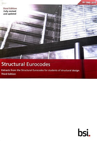
Structural Eurocodes: Extracts from the Structural Eurocodes for Students of Structural Design published by the British Standards Institute.
To help structure the discussion and aid your understanding, we’ll adopt a What, Why, Where and How template:
-
What - A summary of the design check.
-
Where - The relevant clauses within Eurocode 3.
-
Why - Why are we conducting this check?
-
How - A summary of how to conduct the check.
Preliminary step: General description for members under combined bending and axial compression
A steel compression member, depending on whether it falls into the simple column, uniaxial beam-column or biaxial beam-column classification, is subject to a different set of design checks within Eurocode 3. The design checks are split into cross-section resistance checks and member buckling checks.
Helpfully for us, Eurocode 3 provides interaction formulae which are used to assess both cross-sectional resistance and buckling resistance under the combined actions of axial compression and bending.
That said, understanding the nuances of these interaction checks is not so straightforward so we are deliberately starting this design workflow by considering the overarching interaction formulae. It is important that we recognise the 'big picture' before jumping into the detailed design steps.
Note: steel columns are typically class 1 or class 2 sections - (think about how bulky they are!). The following design workflow assumes a class 1 or class 2 section.
What?
For cross-sectional resistance:
where:
is the design plastic moment of resistance when reduced due to the axial force .
For member buckling
For any steel member subject to combined compression and bending, the following two expressions must be satisfied to satisfy member buckling criteria.
where:
are the design values of the compression force and the maximum design moments about the respective axes.
are the moments induced in the section which occur due to the shift of the centroidal axis for class 4 sections.
are the reduction factors which are required to describe flexural buckling (column buckling).
is the reduction factor which is required to assess lateral torsional buckling.
are interaction factors - more on these later!
Where?
- For cross-sectional resistance: EN 1993-1-1: 2005 Clause 6.2.9
- For member buckling: EN 1993-1-1: 2005 Clause 6.3.3
Why?
For cross-sectional resistance
If we think about an elastic stress distribution across a steel section subject to combined axial compression and bending we will recognise that the maximum compressive stress will occur at the extreme fibre of the section where the compressive stresses due to the axial force and the compressive stresses due to the bending moments are combined.
We know from elastic theory that first yield develops when the stress at any point reaches the yield strength of the material, . Put simply, first yield can be reached sooner in sections resisting combined axial compression and bending and we must therefore account for this during design.
Earlier, we said we are considering class 1 or class 2 sections, which can, of course, develop full plastic capacity. This means that the first yielding (as described above) does not constitute section failure.
For member buckling
Looking at the two interaction formulae above we can easily see the relevance of the expressions by breaking down the constituent parts.
Without delving into the intricacies of the interaction factors just yet, we can say that a section under combined axial compression and bending has adequate buckling capacity if:
-
the ratio of design axial force to the flexural buckling resistance , and
-
the ratio of design bending moment about the major bending axis to the lateral torsional buckling resistance , and
-
the ratio of design bending moment about the minor bending axis to the moment of resistance about the minor bending axis , and
-
the sum of the three above ratios
Note: we repeat the above checks for the flexural buckling resistance in both axes.
How?
Throughout the rest of this design workflow, we are going to break down each design step. In essence, we need to obtain the values of all of the constants and variables in the above expressions...so let’s get started!
Step 1: Cross-section classification
What?
In step 1, we need to classify the geometry of the member cross-section. In Eurocode 3, four classifications are defined. The classification is based on the ability of a member to develop its full plastic section capacity. If you have completed the previous tutorial in this series, then these descriptions will be familiar:
-
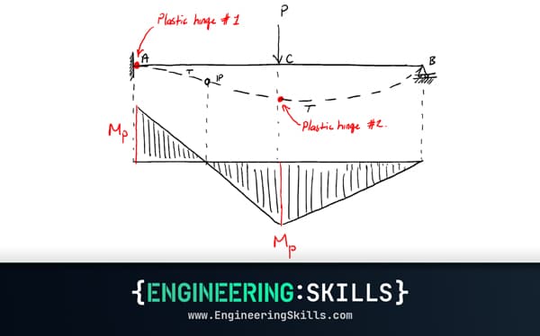
Class 1 cross-sections are those that can form a plastic hinge with the rotation capacity required by plastic analysis without reducing the resistance.
-
Class 2 cross-sections are those which can develop their plastic moment resistance, but have limited rotation capacity because of local buckling.
-
Class 3 cross-sections are those in which the stress in the extreme compression fibre of the steel member, assuming an elastic distribution of stresses, can reach the yield strength, but local buckling is liable to prevent development of the plastic moment resistance.
-
Class 4 cross-sections are those in which local buckling will occur before the yield stress is reached in one or more parts of the cross-section.
Where?
- For the definition of the classes: EN 1993-1-1: 2005 Clause 5.5.2
- For the classification of internal compression parts: EN 1993-1-1: 2005 Table 5.2 (sheet 1 of 3)
- For classification of outstand flanges: EN 1993-1-1: 2005 Table 5.2 (sheet 2 of 3)
Why?
Classifying our cross-section is the method chosen within Eurocode 3 to simplify the analysis of different types of members.
Cross-sections of class 3 and class 4 are susceptible to local buckling failure prior to yielding, whereas cross-sections of class 1 and class 2 are most likely to fail due to the lack of cross-section resistance, as opposed to local buckling.
This simple cross-section classification step allows us to predict the member’s behaviour, and complete the relevant design checks based on the thickness of its constituent parts.
How?
-
Using the diagrams at the top of Table 5.2 (sheet 2 of 3), identify the outstand flange compression parts. For an I-section, this will be the flanges of the member.
-
Calculate the value of , making sure to account for the thickness of surrounding elements and the root radius of any joints.
-
From the section geometry drawing, determine the thickness of the flanges. This is typically for an I-section.
-
Now calculate the value of the quotient for the critical outstand flange.
-
Next, determine the value of by evaluating the quotient where is the yield strength determined in step 1.
-
We are considering a 'part' in pure compression and hence we need to use the left-most column of Table 5.2 (sheet 2 of 3).
-
Now classify the internal compression part of the section by checking if is less than (Class 1), (Class 2) or (Class 3).
-
Now we move on to classify the internal compression parts. For an I-section this is typically the web of the section.
-
Calculate the value of , making sure to account for the thickness of surrounding elements and the root radius of any joints.
-
From the section geometry drawing, determine the thickness of the internal compression parts. Again, this is typically for an I-section.
-
Now calculate the value of the quotient for the internal compression member.
-
We are considering a 'part' in combined bending and compression and hence we need to use the right-most column of Table 5.2 (sheet 1 of 3).
-
To select our limiting values for part classification, we need to calculate , compression proportion of the web.
-
We define as:
-
Using our value of we can compare our value for with the limiting values.
-
Once you have classified both the internal compression parts (the web) and the outstand flanges (the compression flange) then we are ready to classify the section.
-
The overall classification of the section is the lowest of the classifications of the individual parts. For example, if the internal compression part classification is class 3 and the outstand flange classification is class 1, then the section is class 3.
-
You might have guessed this, but if the cross-section parts do not meet the criteria for class 3 then they are class 4. Class 4 steel members are subject to an entire Eurocode 3 document - Eurocode 3: Design of steel structures - Part 1-5: General rules - Plated structural elements. For the time being, we will assume that our section is either class 1, class 2 or class 3.
If you are designing a compression member which does not experience any bending moment, then during classification we would use the table columns from Table 5.2 which correspond to pure compression only. Other than this slight difference, the method is the same.
Step 2: Calculate
What?
Prior to calculating the cross-sectional resistance under the combined action of bending moment and axial force, it is mandatory to first calculate . is the design resistance of the section against axial compressive force - initially as a standalone action.
We don't completely ignore bending moments when calculating since we have assumed a bending stress distribution within the internal compression part (the web) during cross-section classification.
For class 1, 2 or 3 cross-sections, is given by the following:
where is the area of the cross-section.
Where?
EN 1993-1-1: 2005 Clause 6.2.4
Why?
This is perhaps the simplest of all the Eurocode 3 design checks. We calculate the cross-section resistance against axial compression by multiplying the cross-sectional area of the section by the yield strength of the steel. Simple.
How?
This simple check can be completed by following the simple expression shown above. The expression is a little more complicated for class 4 cross-sections but for the time being, we won't concern ourselves with those.
Step 3: Combined cross-section resistance - conservative method
What?
There are a few different approaches which can be taken to assess the cross-sectional resistance under combined bending and compression. We will first consider the conservative approach.
This check simply states that the linear summation of the utilisation ratios of the stress resultants corresponding to the combination of design actions and must be less than unity. The expression we refer to is as follows:
where:
and are the design values of the resistance depending on cross-sectional classification and including any reduction that may be caused by shear effects.
Where?
EN 1993-1-1: 2005 Clause 6.2.1 (7) and Expression 6.2
Why?
This check does exactly what it says on the tin. We are checking that the utilisation ratios for the three leading internal design actions (axial force, major bending and minor bending) are less than unity and that the sum is less than unity. As stated, this is a conservative approach - after all, think about summing three numbers to be less than 1.
How?
- For and , refer to the previous tutorial in this series.
- For , refer to step 3 in this design workflow.
Step 4: Combined cross-section resistance - alternative method
An alternative method (to that covered in step 3) is provided within Eurocode 3. Typically this alternative method results in a more efficient design.
What?
This design check offers a more rigorous approach to assess the cross-sectional resistance against combined bending moments and axial force.
Where?
- Design basis: EN 1993-1-1: 2005 Clause 6.2.9.1
- Interaction criteria for uniaxial bending: EN 1993-1-1: 2005 Clause 6.2.9.1 Expression 6.31
- Interaction criteria for biaxial bending: EN 1993-1-1: 2005 Clause 6.2.9.1 Expression 6.41
Why?
This alternative method is used for the same reason as the method presented in step 3 i.e. ensuring that there is adequate cross-sectional resistance against the combined bending moment and axial compression acting on the section.
How?
For and , refer to the previous tutorial. Once these values are defined, proceed to determine the reduced bending resistance (due to axial force), and using EN 1993-1-1: 2005 Clause 6.2.9.1
For , refer to step 2 in this design workflow.
Step 5: Compression member buckling resistance
What?
Now we move into the more challenging aspect of the Eurocode 3 design checks for beam-columns - member buckling resistance. Once again, we begin with the buckling resistance of the pure compression member. In this design check, we will not be considering the design bending moments - except of course that we maintain the cross-section classification that we obtained in step 1.
Where?
EN 1993-1-1: 2005 Clause 6.3.1.1
Why?
In step 3, we calculated the cross-sectional resistance of a pure compression member. However, as we discussed at the start of this tutorial, cross-sectional resistance is just one part of steel member design to Eurocode 3. We must also consider failure due to member buckling - which can occur at an axial compression force which is much less than the cross-sectional resistance, (again, refer to our tutorial series on theoretical column buckling behaviour or Euler buckling, referenced above).
How?
This is a multi-step design process, so we will break down the compression member buckling resistance check into multiple smaller steps. However, the final expression which we need to evaluate is as follows (for a class 1, 2 or 3 cross-section).
where is the reduction factor for the relevant buckling mode.
Step 5.1 Calculate the non-dimensional slenderness
The non-dimensional slenderness is an indicator of the tendency of a compression member to fail due to flexural buckling. Column sections have a major and a minor buckling axis. As a result, we define two non-dimensional slenderness values, and .
In general, for a class 1, 2 or 3 cross-section, is given by:
where is the elastic critical force for the relevant buckling mode based on the gross cross-sectional properties. An alternative way to express is as follows.
where:
is the critical buckling length i.e. the distance between points of full flexural buckling restraint (for a given axis) and is the radius of gyration - taken about the same axis as and is given by,
So, at the end of this process, we will have two values, and .
EN 1993-1-1: 2005 Clause 6.3.1.2
Step 5.2 Select the buckling curve and find
Now we use Table 6.2 to determine the correct buckling curve. These buckling curves allow us to determine the imperfection factor which we must account for during our flexural buckling check.
Once we know the correct buckling curve, we use Table 6.1 to determine .
EN 1993-1-1: 2005 Table 6.1 and Table 6.2
Step 5.3 Calculate the reduction factor
Now we are at the point where we can calculate the reduction factor . All of the sub-steps we have completed in step 5 have been leading us towards calculating this reduction factor.
First, we calculate as follows:
And using we can now calculate as follows:
Remember that we must complete this calculation for both axes of the section. So by the end of this step you should have two values, and .
EN 1993-1-1: 2005 Clause 6.3.1.2 Expression 6.49
Step 5.4 Calculate the buckling resistance for the beam
We have now calculated our reduction factors and which leaves us to just determine the buckling resistance of the compression member. At this point, we need to choose the critical value for i.e. the largest value, since this will produce the lowest buckling resistance.
where is taken to be in accordance with 6.1 NOTE 2B
EN 1993-1-1: 2005 Clause 6.3.1.1 Expression 6.47
Step 6: Combined buckling resistance
What?
We are now coming towards the end of the Eurocode 3 design checks for a compression member under combined bending and axial force. As we stated at the start of this design workflow, we need to validate the buckling resistance of the member under the action of the combined internal actions.
Recall the expressions:
Which we can simplify as a result of our section being class 1, 2 or 3 down to:
Note: The final component of the two expressions deals with the minor axis bending resistance for the member. You may have noted that on the denominator of the term, we do not apply the reduction factor . This is because members do not exhibit lateral torsional buckling due to bending about the minor axis.
Where?
- For the general expression: EN 1993-1-1: 2005 Clause 6.3.3 Expression 6.61 and 6.62
- _For the factors_: EN 1993-1-1: 2005 Annex A or Annex B - depending on which method is chosen. In this tutorial we will choose Annex A method.
Why?
At this point, it should be clear that the buckling resistance of a member will typically govern the design. In the previous tutorial on steel beam design, we calculated the buckling resistance of members subject to bending moments alone and in step 4 of this article we calculated the buckling resistance of a compression member subject to axial compression only. It will come as no surprise then that the final step of the process is to check the buckling resistance under the combination of both bending and compression.
How?
We are going to use the more exact approach covered in Annex A of Eurocode 3 as it leads to more efficient designs, which in turn, leads to material and cost savings! It should be noted that the simplified approach covered in Annex B is more conservative (and hence still safe to use).
Once again, we are going to break down this Eurocode 3 design check into smaller and more manageable steps.
Step 6.1 Calculate the factor
where
where,
is the St.Venant torsion constant (available in the section tables), is the second moment of area about the major axis and is the non-dimensional slenderness for lateral-torsional buckling due to uniform bending moment i.e. when
Note: head back to step 8.3 and 8.4 in the previous tutorial and calculate for the case when . Once calculated, take .
EN 1993-1-1: 2005 Annex A Table A.1
Step 6.2 Calculate the factor
where
using:
(for class 1, 2 and 3 cross sections)
and
is obtained from Table A.2 using knowledge of the bending moment diagram.
Note:
If
then
EN 1993-1-1: 2005 Annex A Table A.1
Step 6.3 Calculate the factor
where
with coming from Annex A Table A.2 using knowledge of the bending moment diagram for the given axis.
EN 1993-1-1: 2005 Annex A Table A.1
Step 6.4 Calculate the factor
EN 1993-1-1: 2005 Annex A Table A.1
Step 6.5 Calculate the factors
where
EN 1993-1-1: 2005 Annex A Table A.1
Step 6.6 Calculate the interaction factors
We will make the assumption that our section is class 1 or class 2:
where
and
where
Note:
EN 1993-1-1: 2005 Annex A Table A.1
Step 6.7 Evaluate the combined buckling resistance inequalities
All that remains is to plug in all of the calculated values which we have determined in the preceding design steps. If we can show that the value of both inequalities is less than unity then our member has sufficient buckling resistance against the combined bending moments and axial compression.
EN 1993-1-1: 2005 Clause 6.3.3 Expression 6.61 and 6.62
3.0 Steel Column Design - Worked Example
We are now ready to implement our Eurocode 3 design workflow. The worked example deliberately includes as many of the Eurocode 3 column design checks as possible.
Mercifully, most columns do not experience large bending moments, and consequently, many of the design steps will be omitted for simpler design scenarios. Recognising this, section 4.0 will cover a set of simple rules and design simplifications that can be used for the sizing of typical, simple columns.
In each section of the worked example, look out for the references back to the design workflow introduced in the previous section i.e. step 1, step 2, step 3 etc.
3.1 Setting up the problem
In our example problem, we are going to consider a compression member which is subject to bi-axial bending. The characteristics of the problem are as summarised below. Try to think about how these characteristics will inform our selection of Eurocode 3 design checks. The problem is presented with a horizontal member but imagine this member orientated vertically in a structure.
-
The member is subject to an axial force parallel to the -axis - in a structure this axial force would result from gravity loads.
-
The member is subject to a concentrated load acting in the major principal plane i.e. parallel to the -axis.
-
The member is subject to a uniformly distributed load (UDL) acting in the minor principal plane i.e. parallel to the -axis.
-
Lateral deflection and twisting are prevented at both ends of the member and at the midspan point. Other than these points, the member is free to deflect laterally in both planes and to rotate.
3.2 Loading
3.2.1 Permanent Actions ()
- Uniformly distributed load, acting in the positive Y-direction =
- Concentrated Load at Point A in negative Z-direction,
- Concentrated Load at Point B in negative X-direction,
3.2.2 Variable Actions ()
- Concentrated Load at Point A in negative Z-direction,
- Concentrated Load at Point B in negative X-direction,
3.3 Load Cases
3.3.1 Partial factors for actions
- Partial factor for permanent actions, = 1.35
- Partial factor for variable actions, = 1.50
3.3.2 Combination
3.4 Analysis
Now, we progress to the analysis stage, which will allow us to determine the internal actions (against which we will conduct our member design checks). You can use whichever method of analysis you like - we won’t dwell on the method of analysis here.
3.4.1 Applied loads
UDL (self-weight): kN/m
Concentrated Load at A: kN
Concentrated Load at B: kN
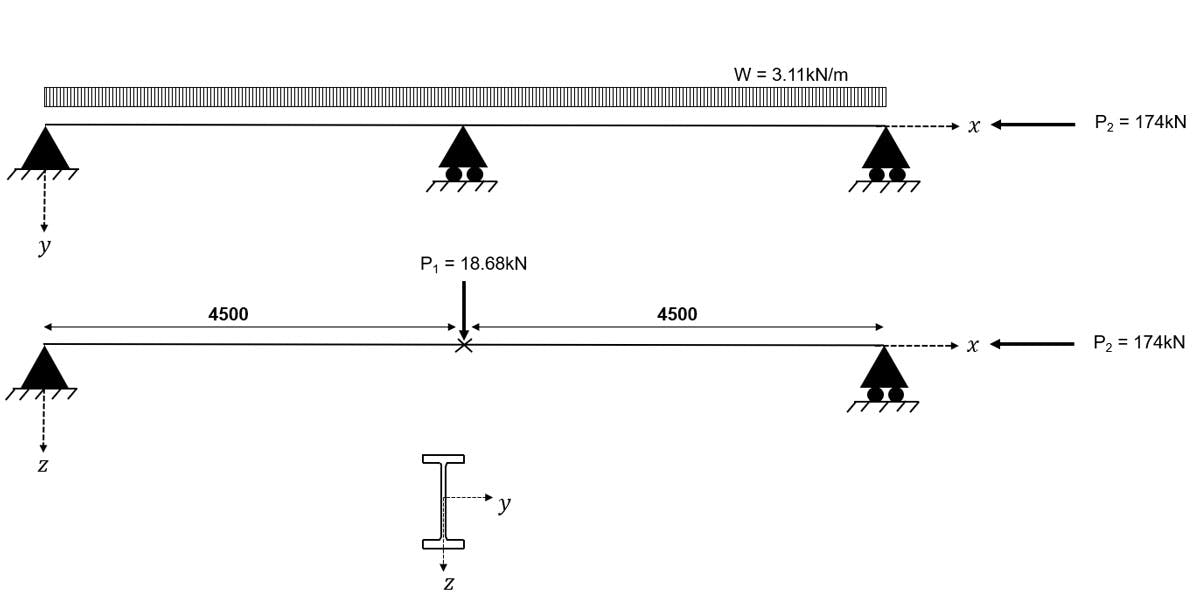
Fig 1. General arrangement of worked example column.
3.4.2 Axial Force
Clearly, the column is subject to an axial compression force of .
3.4.3 Bending moments
As we are considering bi-axial bending, it is necessary to look at bending moment diagrams for both the major and minor axes.
Major axis For the major axis, a single point load at mid-span gives us a simple bending moment diagram with peak value of at mid-span.
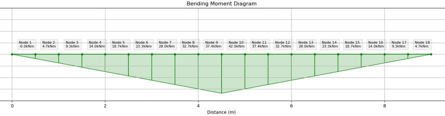
Fig 2. Major axis bending moment diagram.
Minor axis For the minor axis, an additional support is present, which results in a two-span continuous member. The peak moment is a hogging moment located over the central support with a value of .
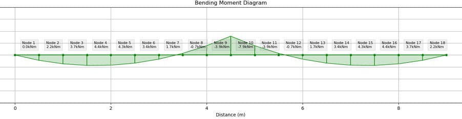
Fig 3. Minor axis bending moment diagram.
3.4.4 Shear Forces
The shear force diagrams are included in this analysis section but we will not be referring to them any further within this tutorial. For beam-columns, the shear forces very rarely govern. In fact, EN 1993-1-1: 2005 Clause 6.2.10 tells us that unless then no reduction to axial or bending resistance. You will find that this clause is met in most cases.
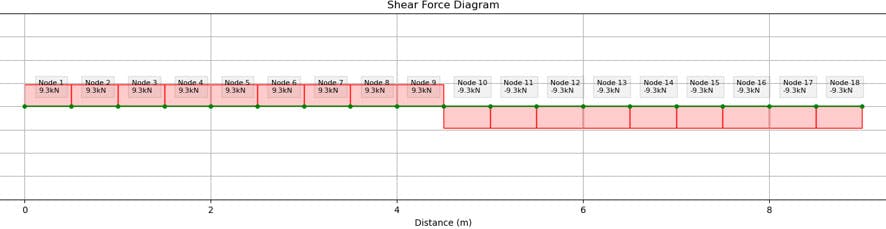
Fig 4. Major axis shear force diagram.
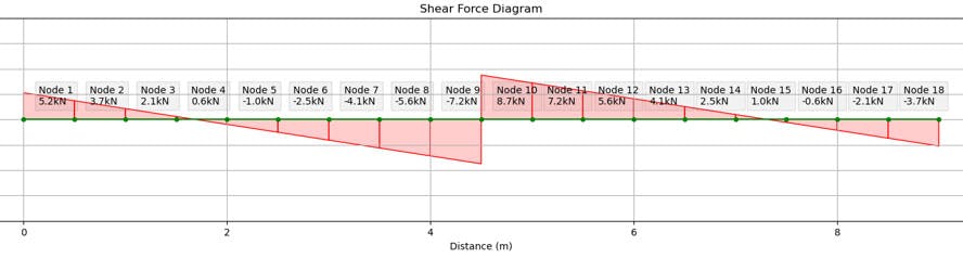
Fig 5. Minor axis shear force diagram.
3.4.5 Deflection
We obtain a separate deflection plot for the major and minor axes. For vertical members such as columns, the lateral deflection is less commonly reported.
However, in Eurocode 3 beam-column design checks, the deflection is used within buckling resistance checks. For that reason, these deflection plots are generated using the ULS combination of loads, rather than the SLS combination.
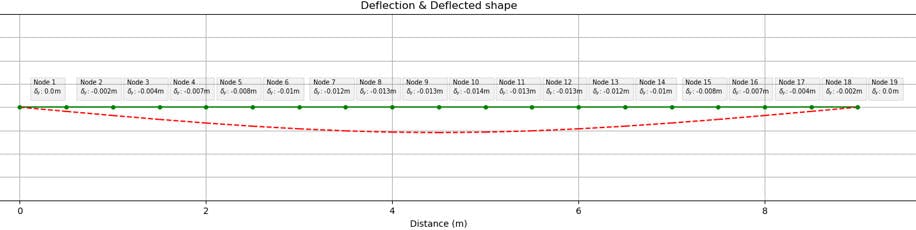
Fig 6. Major axis deflection plot (ULS).
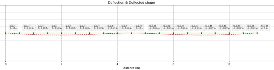
Fig 7. Minor axis deflection plot (ULS).
3.5 Initial section choice
For this worked example, we will try an S355 305x165x46 UB. We’ll discuss some useful tips on the initial sizing of columns and beam-columns at the end of this tutorial. This section is chosen to be quite conservative so that we have some confidence that all design checks will be clearly passed.
From the section properties tables we acknowledge the following:
- Depth,
- Width,
- Web thickness,
- Flange thickness,
- Root radius,
- Depth between fillets,
- Second moment of area about y-y axis,
- Second moment of area about z-z axis,
- Warping constant,
- Torsion constant,
- Radius of gyration about y-y axis,
- Radius of gyration about z-z axis,
- Plastic modulus y-y axis,
- Plastic modulus z-z axis,
- Elastic modulus y-y axis,
- Elastic modulus z-z axis,
- Area,
- Modulus of elasticity,
- Shear Modulus,
Note: the units for each of the above properties are those which are typically used in industry. You will find that using these units is more convenient and avoids using extremely large or small numbers!
3.6 Cross-section classification
Step 1: Determine the yield strength,
- Our section is S355 steel
- We have mm mm
N/mm
EN 1993-1-1: 2005 Table 3.1
Classify the cross-section - Outstand of compression flange
The limiting value for a Class 1 section is . Evaluating the limiting value:
The flange in compression is Class 1.
EN 1993-1-1: 2005 Table 5.2 (sheet 2 of 3)
Classify the cross-section - Web (part subject to bending and compression)
Now given that our part is in combined bending and compression, we first have to calculate
The limiting value for a class 1 internal compression part is:
Evaluating the limiting value:
The section of web in combined bending and compression is Class 1.
EN 1993-1-1: 2005 Table 5.2 (sheet 1 of 3)
Overall classification Both the flange and the web are Class 1. Therefore the overall section classification is Class 1.
3.7 ULS Checks
3.7.1 Cross-section resistance
We have a case of bi-axial bending and hence the following criterion must be used.
where for an I/H section, and where
So in reality, we have to calculate three terms before we can evaluate the criteria for cross-sectional resistance; , and .
Step 2 Calculate
For a class 1 section:
EN 1993-1-1: 2005 Clause 6.2.4
Step 4 Alternative method for cross-section resistance
To make our design checks simpler, we enlist two specific clauses from Eurocode 3.
EN 1993-1-1: 2005 Clause 6.2.9.1 (4) tells us that:
for doubly symmetrical I- and H-sections or other flanges sections, allowance need not be made for the effect of the axial force on the plastic resistance moment about the y-y axis when both the following criteria are satisfied:
and
so we proceed to test these two criterion:
and
So both criteria are met, which means that we can say the following for the plastic moment resistance about the y-y axis.
EN 1993-1-1: 2005 Clause 6.2.9.1 (4) tells us that:
for doubly symmetrical I- and H-sections, allowance need not be made for the effect of the axial force on the plastic resistance moment about the z-z axis when:
so we proceed to test this criterion:
The criterion is met, which means that we can say the following for the plastic moment resistance about the z-z axis.
Now we can re-visit the governing criterion:
Therefore the cross-section is adequate when we consider the combined actions of axial compression and bi-axial bending.
3.7.2 Buckling resistance
Step 5: Compression member buckling resistance
Before we progress with determining the combined buckling resistance of the member, we first need to determine the buckling resistance of the member, assuming it sees only axial compression.
Step 5.1 Calculate the non-dimensional slenderness
We define two non-dimensional slenderness values, and .
where:
EN 1993-1-1: 2005 Clause 6.3.1.2
Step 5.2 Select the buckling curve and find
For and mm, we consider the following:
- For buckling about the axis, use buckling curve a, so take
- For buckling about the axis, use buckling curve b, so take
EN 1993-1-1: 2005 Table 6.1 and Table 6.2
Step 5.3 Calculate the reduction factor
Now we are at the point where we can calculate the reduction factor . Recall that we need to calculate this for buckling about both axes.
First, we calculate as follows:
And using we can now calculate as follows:
EN 1993-1-1: 2005 Clause 6.3.1.2 Expression 6.49
Step 5.4 Calculate the buckling resistance for the beam
where is taken to be in accordance with 6.1 NOTE 2B
So we can say that the buckling resistance, , is therefore, for the case of axial compression only, the member has adequate buckling resistance.
EN 1993-1-1: 2005 Clause 6.3.1.1 Expression 6.47
Step 6: Combined buckling resistance
Step 6.1 Calculate the factor
We break this expression down and calculate the individual terms one by one.
To calculate and we need to utilise the design checks we covered in our steel beam design tutorial. If you need to refresh yourself on these design checks, review that tutorial first. In this example, we’ll move swiftly through these results.
We have a section with and mm and so choose LTB buckling curve a - therefore
We can now come back and calculate
Step 6.2 Calculate the factor
Once again, we break this expression down and calculate the individual terms one by one.
Now we need to determine . The first step in this is to evaluate the inequality as follows:
therefore
using:
and returning back to the original expression for
Step 6.3 Calculate the factor
Again, let us state what we know first.
So all that remains is to determine
where
and
Now revisiting the original expression for
Step 6.4 Calculate the factor
Step 6.5 Calculate the factors
Evaluating
Evaluating
Evaluating
Evaluating
where
Step 6.6 Calculate the interaction factors
Noting that our section is class 1:
where
and
where
Step 6.7 Evaluate the combined buckling resistance inequalities
All that remains is to plug in all of the calculated values which we have determined in the preceding steps. If we can show that the value of both inequalities is less than unity then our member has sufficient buckling resistance against the combined bending moments and axial compression.
Since both inequalities have been satisfied, we have shown that the two governing criteria are met and therefore the proposed section has adequate buckling resistance against the combined action of axial compression and bi-axial bending. In fact, the utilisation is around 60% and therefore if we wanted to, the section size could be further optimised.
4.0 Initial sizing of compression members
The previous design example demonstrates the potential complexity involved in designing compression members to Eurocode 3. The chosen design example aimed to be as broad as possible to allow a full breadth of design checks to be conducted.
In reality, most columns are simple, as explained at the start of this tutorial. As a result, we can greatly simplify the design checks involved.
4.1 Simplified approach for simple columns
We can simplify the governing buckling criteria for simple columns down to the following expression
Which I am sure you will agree is much simpler than the two buckling criteria we used in our worked example.
A further simplification can be afforded by taking . So, in reality, a simple column can be designed in two steps:
- Check the combined resistance using the following:
- Check the combined buckling resistance using the following:
If we step back and look at these expressions, the only term which we need to perform multiple calculation steps on is - and we know from the worked example that this is one of the simpler Eurocode 3 calculations.
To make your life even easier, you can make an initial assumption that = 0.7, which allows a section to be chosen on the basis of area alone, using the following expression.
Once you've picked your section, then the above two criterion can be checked reasonably quickly.
5.0 Wrapping up and Coming up next
I hope you have found this tutorial on the design of steel compression members to Eurocode 3 helpful. This tutorial is intended to give you the skills and confidence to use Eurocode 3 Part 1-1 to design steel compression members, including those which must resist bi-axial bending in addition to axial compression. You should now have a good understanding of the different design checks which we conduct and the reason why we conduct them.
In our next tutorial in this series, we focus our attention on the design of steel trusses. As we know, Eurocode 3 does not have specific sections for this type of application and instead categorises members based on the internal forces which they must resist...can you think which internal forces we will be considering for steel members within truss structures?
We will answer all of these questions, and quite a few more, in the next instalment.

Featured Tutorials and Guides
If you found this tutorial helpful, you might enjoy some of these other tutorials.

A Pynite Crash Course - Open Source Finite Element Modelling for Structural Engineers
Part 1 - Get hands-on with V1.0 of this exciting new Python FEA library

Dan Ki