Structural Analysis and Stability – Symmetrical Structures

All structures typically experience some form of lateral loading during their design life. Typical sources of lateral loading include forces due to wind blowing against the structure, hydrostatic forces due to groundwater (acting against basement walls for example) or inertia forces due to ground motion (earthquakes).

The designer must consider how to transmit these lateral loads safely back into the foundations of the structure. In the context of building structures, there are several well established structural schemes for facilitating this load transfer. In this, the first of a two-part series on structural stability, we will introduce these schemes before diving into some numerical examples in this and the next post.

Structural Stability of Braced Structures

Consider a basic structural frame subject to a single lateral load, $P$ ,

Structural Analysis and Stability - An unbraced structures

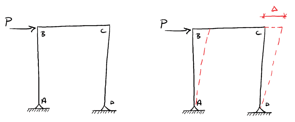
Fig 1. (Left) Simple frame subject to a lateral load $P$ . (Right) Sway deflection $\Delta$ resulting from $P$ .

Under the action of the load, the frame will deflect to the right by an amount denoted by $\Delta$ . This deflection occurs due to:

rotation of the structural members relative to each other at joints B and C.
bending of the vertical members.

One of the simplest ways to reduce the degree to which the frame deflects is to provide a diagonal member, ‘triangulating the frame’. Depending on the orientation of the diagonal bracing member (relative to the direction of the external loading), it may develop a compression force (referred to as a strut) or a tensile force referred to as a tie, So, for any lateral deflection to occur, the diagonal member must get longer or shorter depending on its orientation.

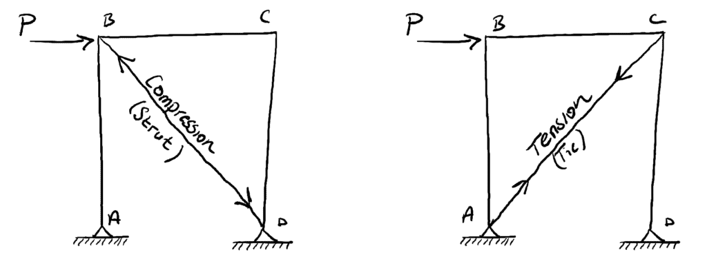
Structural Analysis and Stability - Strut and Tie bracing

Fig 2. (Left) Braced frame with compression developing in the bracing strut. (Right) Braced frame with tension developing in the bracing tie.

The design of a (compression) strut involves the additional consideration of buckling and so if all else is equal, structural (tension) ties tend to be more efficient. The preference for ties over struts is apparent when we see ‘cross-bracing’ consisting of slender structural ties.

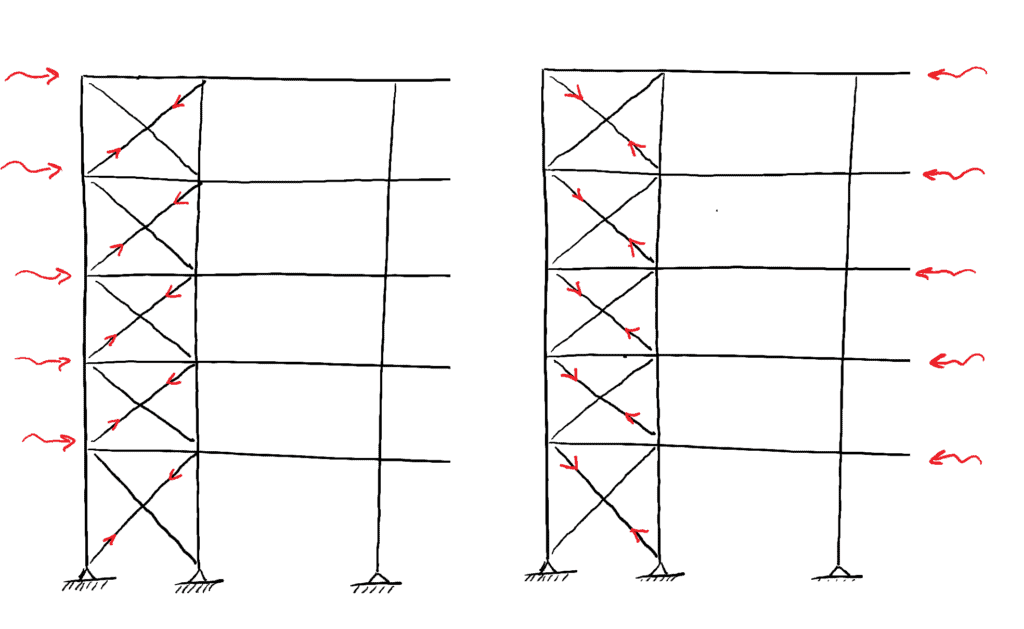
Structural Analysis and Stability - multi-storey tie bracing

Fig 3. Cross-bracing in a multi-storey structure utilising only tension members.

In such cases, depending on the direction of loading, one member will be ‘active’ and in tension while the other member is dormant not providing any resistance to lateral loading. If the external load direction reverses as seen on the right in the image above, the ties switch roles; the dormant member becoming active and vice-versa.

Structural Stability of moment or portal frames

When considering our simple frame structure above, for a deflection to occur, we said that the angles between the vertical members and the horizontal member at joints B and C must change. Another way to reduce the amount of lateral frame deflection is to reduce the amount of relative rotation at these joints. In other words, by stiffening the joints and increasing their resistance to rotation, we reduce the overall lateral deflection of the frame.

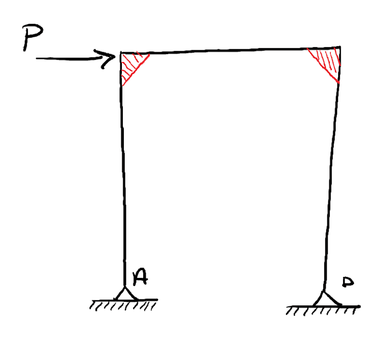
Structural Analysis and Stability - portal frame

Fig 4. Schematic view of a portal frame with stiffened joints indicated in red

A structural frame in which the resistance to lateral loading is provided by the beam to column connections is called a portal frame. Joint stiffness is enhanced by providing ‘haunches’ that serve to increase the lever arm available at the joint, (below). Haunches also reduce the effective span of the members between joints.

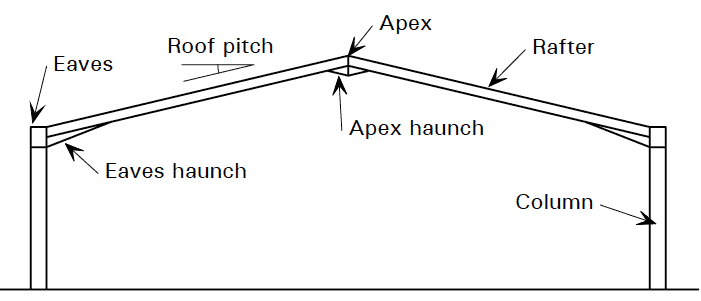
Fig 5. Typical symmetrical portal frame.

Portal frame structures are most often encountered as steel frame structures, e.g. large warehouses, agricultural buildings, hangers. Portal frames are characterised by their ability to span large distances efficiently. In doing so they typically make use of plastic hinge formation. Lateral deflection of portal frames is largely dependent on the stiffness of structural joints and also the flexural rigidity of vertical (column) members. The result of this is that portal frames generally experience larger lateral (sway) deflections than braced frames.

Stability of Propped Structures

The third stabilising mechanism and the one we will explore in more detail in this series of posts is the so-called propped structure scheme, regularly employed in multi-storey frame structures, e.g. reinforced concrete (RC) frame buildings. In multi-storey RC frame buildings it’s common for concrete lift and stair shafts (also known as cores) to act like vertical cantilevers, providing the building’s resistance to lateral loads such as wind.

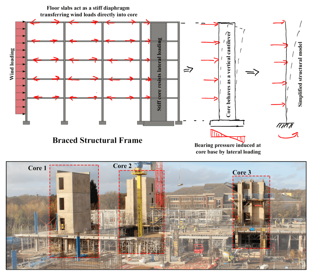
Fig 6. Cantilevering concrete cores providing lateral stability in an RC frame structure.

In this case the combined stiffness of the cores is significantly greater than the lateral stiffness provided by the column-beam connections. As a result the RC walls of the cores ‘attract’ or resist the majority of the lateral force imposed by wind for example. Such a building is said to be propped by the cantilevering cores. Vertical shear walls serve the same function.

Look around any large site with multi-storey structures and there is a strong possibility you will see this stabilising mechanism. Also note that the RC cores are constructed ahead of the floors and tower over the structure below. This is because they provide the stiff points within the structure with all other structural elements (beams and floor slabs) being propped against them.

In order to utilise the RC cores as stabilising elements, the lateral forces (say the wind blowing on the facade) must be transmitted back into the core. This is achieved by utilising the floor slabs (also known as floor plates) as stiff diaphragms. This can be seen in the diagram, above, with the red arrows indicating compression force transmission through the floor slabs back to the cores. Along the line of action of the horizontal compression forces (from the facade), the floor plates are exceptionally stiff and provide an ideal load path back into the cores.

Stability of a Symmetrically Propped Structure

To develop our understanding of this stability scheme, we will consider the case study structure, pictured below. This RC frame consists of a ground floor (not shown) and 6 floor slabs (shown in green). Indicative finished floor levels (FFL) are also indicated. The stabilising elements are shown in red and consist of two shear walls and a central core. The columns provide for vertical load transmission only and do not contribute to lateral stability. The bottom image also shows a typical floor plan with dimensions indicated. We will assume a design wind loading of 1.2 $kN/m^2$ from the south. Our task is to estimate the stresses induced at the base of the stabilising elements. As you will see, this can be accomplished by utilising quite rudimentary analysis techniques. We will assume all RC walls are 400 mm thick and the core is located centrally on the floor plan.

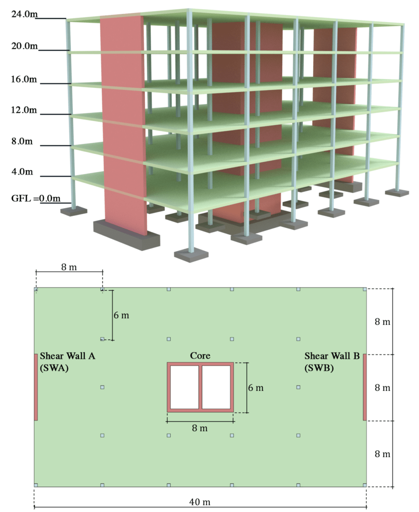
Structural Analysis and Stability - symmetrically propped structure example

Fig 7. (Top) A multi-storey reinforced concrete frame building stabilised by shear walls and central core (red). Stiff floor plates (green) provide a load path from facade back into vertical stability elements. (Bottom) Typical floor plan.

Our first task is to determine the total wind loading acting on the building facade:

\begin{align*} F_{wind} &= 40\:\textup{m} \times 24\:\textup{m} \times 1.2\:\textup{kN/m}^2\\ &=1152 \:\textup{kN} \end{align*}

This force must be distributed between the three stabilising elements in proportion to their stiffness or flexural rigidity, $EI$ . Since all members are made of the same material, we can focus on their second moment of area:

I=\frac{bd^3}{12} \tag{1}

Since it is only the relative stiffness that is important we can evaluate only the numerator since the denominator is common to all. This relative stiffness will be denoted as $\hat{I}$ . Evaluating the shear wall relative stiffness:

\begin{align*} \hat{I}_{swa} &= \hat{I}_{swb} = 400\times8000^3\\ &=2.048\times10^{14}\:\textup{mm}^4 \end{align*}

Note that the shear walls act to resist lateral loading in the north-south direction only. In the east-west direction the shear walls have negligible stiffness (in comparison to their stiffness in the north-south direction).

The relative stiffness of the core can be determined by first calculating $\hat{I}$ for the outer enclosing rectangle and then subtracting $\hat{I}$ for the two voids:

\begin{align*} \hat{I}_{core} &= \hat{I}_{out} - \hat{I}_{in}\\ &=(8000\times6000^3)-2(3400\times5200^3)\\ &=7.719\times10^{14}\:\textup{mm}^4 \end{align*}

After determining the relative stiffness of each active element, we can distribute the lateral load, $F_{wind}$ , accordingly:

\begin{align*} F_{swa} = F_{swb} &= \frac{\hat{I}_{sw}}{\sum \hat{I}}\times F_{wind}\\\\ &=\frac{2.048\times10^{14}}{11.815\times 10^{14}}\times 1152\\\\ &=199.7\:\textup{kN}\approx 200\:\textup{kN}\:\: \textup{say} \end{align*}

Therefore, $F_{core} = 1152\:\textup{kN} - 2(200) = 752\:\textup{kN}$ . Perhaps not surprisingly, the central core is resisting the largest proportion of the external wind loading in the north-south direction.

We can repeat the same exercise now assuming wind acting in the east-west direction. As mentioned above, in their current orientation, the shear walls provide negligible resistance to external loading in this direction. This is confirmed by evaluating the relative stiffnesses:

\begin{align*} \hat{I}_{swa} = \hat{I}_{swb} &= 8000\times400^3\\&=5.12\times 10^{11}\:\textup{mm}^4\\ \hat{I}_{core}&=6000\times 8000^3 - 2(5200\times 3400^3)\\ &=2.663\times10^{15}\:\textup{mm}^4 \end{align*}

By inspection we can see that the core will resist in excess of 99% of the external loading due to its much larger relative stiffness. By visualising the shear walls in isolation and considering them as simple cantilevers we can easily see the importance of the axis of bending.

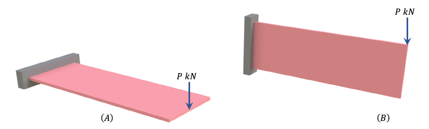
Structural Analysis and Stability - shear wall axes

Fig 8. The structure on the left (A), is said to be bending about its minor or weak axis, while the structure on the right is bending about its major or strong axis. Intuitively we would expect (B) to provide significantly more resistance to the load, $P$, than (A). This is what we have seen in the previous example.

Now that we have a model of the lateral load distribution in the structure, it is a relatively straightforward exercise to estimate the stresses that develop at the base of the shear walls and core. By way of demonstration, we will consider the stress that develops at the base of one of the shear walls in response to wind loading from the south.

Our previous analysis suggests one shear wall resists approximately 17.3% of the wind load or $200 kN$ . This is transmitted back into the wall via 6 floor plates, with the top floor (roof) transmitting half the magnitude of any of the lower floors, thus we can say, $5.5\:P=200\:kN$ . Therefore $P=36.4\:kN$ and the load distribution can be modelled as shown below.

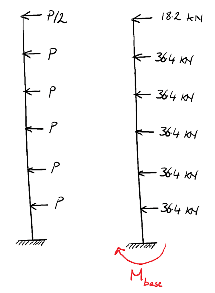
Structural Analysis and Stability - load distribution from floors

Fig 9. Distribution of floor loading into one shear wall

By modelling the load distribution onto the wall, we can determine the bending moment generated at the base of the wall, $M_{base}$ . It is then a trivial exercise to use the engineer’s bending equation to evaluate the corresponding stress. We can determine the bending moment at the base as the sum of the individual bending moments generated by each force, so;

\begin{align*} M_{base} &= 36.4\times 4 \\ &+ 36.4\times 8 \\ &+ 36.4\times 12 \\ &+ 36.4\times 16 \\ &+ 36.4\times 20 \\ &+ 18.2\times 24 \\\\ M_{base} &=2620.8\:kNm \end{align*}

We can evaluate the second moment of area for the wall’s cross section as:

\begin{align*} I&=\frac{400\times 8000^3}{12}\\ &=1.707\times 10^{13}\: \textup{mm}^4 \end{align*}

Assuming the wall’s neutral axis is coincident with its centroid, the maximum tension and compression stress will occur at a distance of $y=4000\:$ mm from the neutral axis, therefore the maximum axial stress that develops at the base of the wall is given by:

\begin{align*} \sigma_{max} &= \pm \frac{M_{base}\:y}{I}\\ &=\pm \frac{2620.8\times 10^{6}\times 4000}{1.707\times 10^{13}}\\ &=\pm 0.61\:\textup{N/mm}^2 \end{align*}

So our analysis suggests that the maximum tensile stress that will develop is $0.61\: \textup{N/mm}^2$ . If we assume the walls are constructed with concrete with a characteristic cylinder strength $f_{ck}=30\:\textup{N/mm}^2$ , an approximate estimate of the tensile capacity of the concrete would be $2.5-3.0 \textup{N/mm}^2$ . Therefore we would not expect the wind loading to cause tension cracks at the base of the wall. Furthermore, when we factor in the self-weight of the wall and any additional compression stresses due to floor loadings, the tensile stress developed due to wind loading is easily accommodated. A similar exercise can be completed to confirm the acceptability of stresses developed in the core walls.

The the next post we’ll consider how this analysis plays out for asymmetrically propped structures and confirm the results of our hand analysis with a simple FE model analysis.