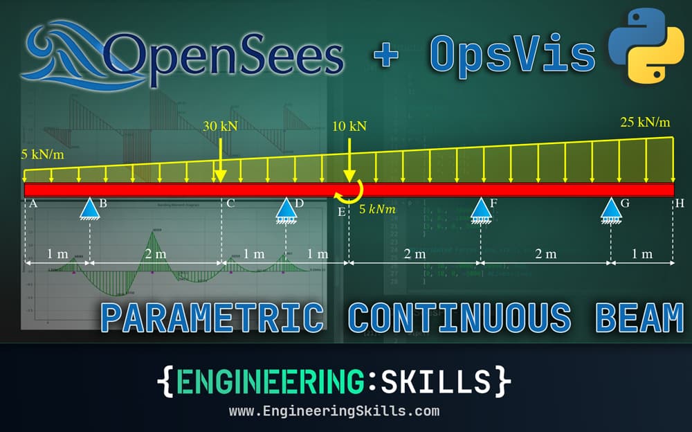
Build a Parametric Continuous Beam Calculator using OpenSeesPy

1.0 Introduction

In this short tutorial, we’ll build a continuous beam analysis script using OpenSessPy. Multi-span continuous beams are so common, that it makes sense to have a script in our toolbox to very quickly generate the shear force diagram, bending moment diagram, reactions and deflected shape.

Analysing them by hand takes forever and even setting them up for analysis in commercial software packages can feel laborious. This is where having a simple analysis script comes in handy - quickly plug in the beam parameters, hit Run and you’re done!

Once you complete this tutorial, you’ll have built this script. Work through it with me now, step-by-step or download the completed code from the resource panel above.

This is the third in our series of tutorials exploring the OpenSeesPy library. If you’re completely new to OpenSeesPy, go back to the first tutorial here, where I introduce the library.

This continuous beam project follows on very closely from part two in the series where we analysed a 2D moment frame. Make sure to check that out before you work through this. In fact, the OpenSeesPy portion of the build will be almost exactly the same - what’s new in this tutorial is how we handle some of the structure parameterisation.

Our plan will be to define the structural parameters (material, geometry and loading) first. Then we’ll dive into building the OpenSeesPy model, tackling the parameterisation as we define various parts of the model.

Ok, let’s get into the build!

2.0 Parameterising the Continuous Beam

Our goal is to have the entire definition of the structure parameterised. All this really means is that we want to be able to define everything at the start of the script and then let the code handle the OpenSeesPy model building process.

We can start by defining the material and geometric properties of the cross-section:

Young’s Modulus for the beam material (we’ll assume steel), $E$
Cross-sectional area of the continuous beam section, $A$
Second moment of area about the major principle axis of the section, $I_z$

#Constants
E = 200*10**9   #(N/m^2) Young'Modulus
A = 0.03        #(m^2) Cross-sectional area
Iz = 300*10**-6 #(m^4) Second moment of area

We’ll define the overall span of the beam next. Note that this is the entire beam length and ignores the positions of supports. We’ll start by assuming a $10\:m$ beam.

L = 10 #(m) Total beam length

Next we define the positions of supports as well as the degree of restraint provided by each. The data for one support will be stored in a list consisting of 4 numbers:

The first number indicates the location of the support
The second indicates the whether or not the support provides horizontal translational restraint
The third indicates the whether or not the support provides vertical translational restraint
The fourth indicates the whether or not the support provides rotational restraint.

Restraint is indicated by the number 1 with no restraint indicated by 0. So for example, [1, 1, 1, 0] defines a pin support located $1\:m$ along the beam, assuming the origin is at the left-most tip if the beam.

We can collect all support data lists into another list. So, in ur case we define 4 supports as follows:

#Restraints [pos, Ux_Restraint, Uy_Restraint ThetaZ_Restraint]
r = [
    [1, 1, 1, 0], #Pin
    [4, 0, 1, 0], #Roller
    [7, 0, 1, 0], #Roller
    [9, 0, 1, 0], #Roller
    ]

We take a similar approach when defining the loading information. Each action on the structure is defined by a list of numbers with all actions applied to the structure being collected into a single list. We define point actions (point moments and forces) first,

#Point Forces and Moments [pos, Fx, Fy, Mz]
p = [
    [3, 0., -30000., 0.],
    [5, 0., -10000., 0.],
    [5, 0., 0., 5000.]
    ]

Distributed loads are similarly defined. Note that we can define both uniformly distributed loads and loads of linearly varying intensity, by specifying a different beginning and ending intensity.

#Distributed Forces [pos_start, pos_end, intensity_start, intensity_end]
w = [
    [0, 10, -20000, -20000], #UDL
    [0, 10, 0, -5000] #Linear Load
    ]