Building a Parametric Frame Analysis Pipeline with OpenSeesPy and OpsVis
![[object Object]](/_next/image?url=%2Fimages%2Fauthors%2Fsean_carroll.png&w=256&q=75)
...we’ll build a pipeline for the elastic analysis of a 2D portal frame structure using OpenSeesPy. Along the way,
- we’ll parameterise our code so we can specify the bay width and number of bays at the start of our pipeline.
- we’ll use another library, OpsVis, to visualise our model and results without having to write our own plotting code.
By the end of this tutorial, you’ll understand how to do 2D frame analysis with OpenSeesPy and be comfortable expanding the code for more complex 2D structures.
1.0 Introduction
Welcome to this second tutorial in our series focusing on OpenSeesPy. If you missed the first tutorial - where we introduced OpenSees, OpenSeesPy and built a truss analysis code, check that out here.
In this tutorial, we’re stepping up the complexity of the structure we’re going to analyse. Here, we’re focussing on the elastic analysis of a 2D portal frame. It's not the most complex thing we could tackle. Still, it's definitely a step up from a truss - and sufficiently common that having a quick way to perform the analysis with OpenSeesPy will actually be a real asset to you!
So, in this build, we’re dealing with elements that can develop a resistance to transverse shear forces and bending moments, in addition to axial forces. We’ll also have three degrees of freedom per node rather than two. This introduces one or two extra details into the mix, but it’s actually remarkable how similar this code will be to our previous truss analysis code.
You’ll see that I’m using the term pipeline to describe the code we’ll build - this is because when we use OpenSeesPy to analyse our model, we go through a fairly predictable (and repeatable) series of steps.
We never really need to dig into the underlying mechanics. We let OpenSeesPy handle that for us - which is fine if you already understand the nuts and bolts of how it all works, behind the scenes. For me, this brings up the notion of a conveyor belt or pipeline where, at each stage, we’re performing a relatively simple, discrete operation.
This is in contrast to building the code from the ground up without making use of specialist analysis libraries. Probably the best way to fully understand what a tool like OpenSeesPy is doing is to first go through the process of building something similar yourself…(you can see where this is going!!)...which is what we do in our course, Beam and Frame Analysis using the Direct Stiffness Method in Python. If you want to fully understand what OpenSeesPy is doing for you - this course will walk you through the process of building a feature-complete 2D frame analysis solver - with all of the underlying mechanics fully explained.
Beam and Frame Analysis using the Direct Stiffness Method in Python
Build a sophisticated structural analysis software tool that models beams and frames using Python.
After completing this course...
- You’ll understand how to model beam elements that resist axial force, shear forces and bending moments within the Direct Stiffness Method.
- You’ll have your own analysis software that can generate shear force diagrams, bending moment diagrams, deflected shapes and more.
- You’ll understand how to model rotational pins within your structures, inter-nodal distributed loading and realistic flexible supports.
1.1 OpsVis
OpenSeesPy is a powerful tool, but one of its Achilles heels, certainly from the point of view of adoption, is the fact that there is no built-in way to visualise your results graphically. This means you need to build your own data extraction and plotting code like we did in the previous tutorial or find a library that plays nicely with OpenSeesPy!
That’s where OpsVis comes into the picture. OpsVis is a separate library built specifically to work with OpenSeesPy. Here’s a video of the main developer, Dr. Seweryn Kokot talking about the library.
Rather than writing our own code, we’ll use OpsVis to plot:
- our structure and loading to make sure everything has been defined correctly
- the deflected shape
- the bending moment diagram
- the shear force diagram
- the axial force diagram
Although we’ll sacrifice a certain degree of customisation and flexibility by not writing our own plotting code from scratch - this will be a lot faster.
If you’ve completed the previous tutorial, you will already have OpenSeesPy installed on your machine - as a reminder, just execute...
pip install openseespy
...in your terminal if you’re on a Mac. You’ll need to do the equivalent installation on Windows.
To download and install OpsVIs, execute...
pip install opsvis
2.0 Analysis Case Study
The structure we’ll analyse is Test Question 4, taken from lecture 53 of Beam and Frame Analysis using the Direct Stiffness Method in Python. We’ll briefly review the structure and its elastic behaviour before building our OpenSeesPy pipeline.
Basing our analysis on this structure also means we have something to validate our OpenSeesPy results against - critical when we’re building a new code or working with a new library. The risk is not so much that the library will produce an error, but that we will make an error implementing some feature or method from the library. So a reliable ground truth model is really helpful.
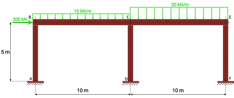
Fig 1. Analysis case study: Single-storey two-bay portal frame with externally applied loading.
Our structure is a two-bay, single-storey portal frame. We’ll parameterise our code so that we can easily modify the bay width and number of bays. This is really just to demonstrate the power of parameterisation. You can expand this and parameterise as much as you like - why not add in a parameter for the number of storeys for example…go wild!
Our frame is subject to a combination of uniformly distributed and point loads, applied both horizontally and vertically and has built-in or cantilever supports at the base.
2.1 Elastic versus plastic analysis
It’s worth making a quick note here on the fact that we’ll be performing an elastic analysis. This means that all members are assumed to remain within their elastic limit. This contrasts with how structures like this are often designed in practice - using plastic analysis. In fact, we have a full tutorial on the plastic analysis of frames. You can check that out to learn more.
In a nutshell, a plastic analysis would allow us to produce a more efficient design since we would allow for the development of plastic hinges in the structure. This would mean we could apply more load to the structure before it exceeds its failure criterion.
Hinge formation is facilitated by the fact that our frame is statically indeterminate and can accommodate the formation of a fixed number of hinges before the collapse occurs. When executed carefully and correctly, this is a perfectly acceptible design practice and will yield more efficient designs. We can perform this type of analysis with OpenSeesPy, but that's a story for another day - we’ll stick with our elastic analysis for now.
2.2 Structural behaviour
When we analyse this structure in our custom code, developed during our Beam and Frame Analysis using the Direct Stiffness Method in Python course, we obtain the following results.
Deflection and Deflected Shape
The following plot shows the deflected shape of the structure with labels added to show the lateral deflection at each node. The lateral deflection at the eaves is 0.019m. Note that the deflected shape has been scaled by a factor of 50.
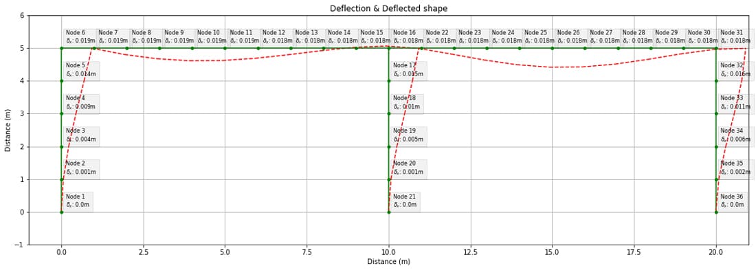
Fig 2. Case study structure deflected shape from course code.
Bending Moment Diagram
Next, we have the bending moment diagram with labels selected to show the bending moment at node i of each element. We’ll return to the specific values later when we directly compare to our OpenSeesPy results.
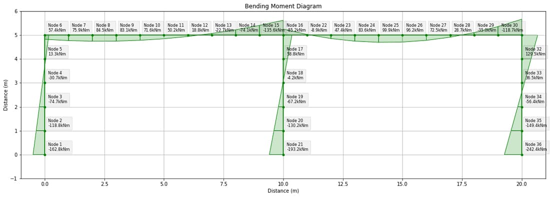
Fig 3. Case study structure bending moment diagram from course code.
Shear Force Diagram
The shear force diagram is shown below. Again, labels have been selected so show the shear force value at node i of each element.
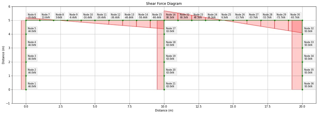
Fig 4. Case study structure shear force diagram from course code.
Axial Force Diagram
Finally, we can summarise the axial forces with the labelled diagram below.
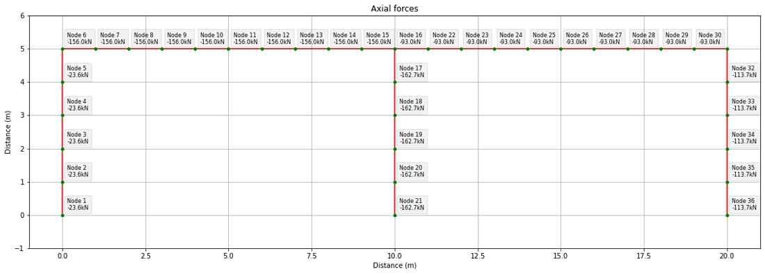
Fig 5. Case study structure axial force diagram from course code.
3.0 OpenSeesPy Analysis
Now that we’ve summarised the case study structure and its elastic behaviour, we can start building our OpenSeesPy analysis pipeline. As I said in the previous tutorial, when building out an analysis code like this, it’s essential to reference both the OpenSeesPy documentation and the original OpenSees documentation here and here. With these resources, you can, pretty much, piece together whatever you’re trying to accomplish. Of course, you’ll also need to refer to the OpsVis docs when dealing with that library.
3.1 Imports and defining constants
As usual, we start by importing our libraries…all the usual suspects. Note the additional import of opsvis - this is a new one for us.
#OpenSeesPy and Opsvis
from openseespy.opensees import *
import opsvis as opsv #For OpenSeesPy visualisation

import math
import numpy as np
import matplotlib.pyplot as plt
Next, we can define our constants, geometric parameters and base fixity.
#Constants
E = 200*10**9 #(N/m^2) Young'Modulus
A = 0.03 #0.01 #(m^2) Cross-sectional area
Iz = 300*10**-6 #(m^4) Second moment of area

#Geometry parameters
nBays = 2 #Number of bays
h_bay = 5 #(m) #Portal height
w_bay = 10 #(m) #Portal width

#Support fixity
fixity = (1,1,1) #Three degrees of freedom (tx, ty, rz) all fixed
The fixity variable will be used later. But (1,1,1) indicates fixity for each of our three degrees of freedom (built-in support).
3.2 OpenSeesPy - Initialisation
Next, we can call the wipe() method to clear any pre-existing models from memory and initialise our model by specifying the dimensionality of the problem and the number of degrees of freedom per node - three this time, , , and .
# Remove any existing model
wipe()

# Initialise the model - 2 dimensions and 3 degrees of freedom per node
model('basic', '-ndm', 2, '-ndf', 3)
3.3 OpenSeesPy - Structural Model Definition
When we defined our truss model in the previous tutorial, we manually specified the nodal positions and the connectivity matrix. We could do this again, but since we’ve decided to parameterise our model, we’ll use these parameters when defining nodes and elements. It’s easier than it might sound - let’s start by defining the nodes.
Nodes
We know that the number of columns will be equal to the number of bays + 1 (nBays+1), so we can implement a for loop to cycle through each column and define the node at the base and at the eaves, in turn.
The node definition uses the command we’ve seen previously, node() with the node tag, x-coord and y-coord passed in. Here’s the complete code block:
#Cycle through columns and define nodes at base and eaves
for i in range(nBays+1):
    index=i+1 #Want iterator to start at 1 not zero (personal preference :)
    xCoord = i*w_bay

    #Base nodes
    nodeTag = (2*index)-1
    yCoord = 0
    node(nodeTag, xCoord, yCoord)
    print(f'Base node with tag {nodeTag} defined')

    #Eaves nodes
    nodeTag = (2*index)
    yCoord = h_bay
    node(nodeTag, xCoord, yCoord)
    print(f'Eaves node with tag {nodeTag} defined')
Visualising our nodes with OpsVis
This is where OpsVis comes into play. At this point it would be good to visualise our newly defined nodes to make sure everything went according to plan. OpsVis offers us a quick way of doing this - the plot_model() function.
Now, since we’re going to visualise our model multiple times throughout this pipeline, we can wrap our OpsVis plotting code inside a function. We’ll add in some housekeeping commands to tidy up our plot too.
def plotStructure(title):
    #Pass in optional argument (fig_wi_he) to control plot size
    opsv.plot_model(fig_wi_he=(50,20))

	#Housekeeping
    plt.title(title)
    plt.xlabel('Distance (m)')
    plt.ylabel('Distance (m)')
    plt.grid()
    plt.show()
Our plotStructure() function also takes a title so that we can customise the resulting plot title each time we call the function. Now we just need to actually call the function we’ve defined.
plotStructure('Frame Nodes')
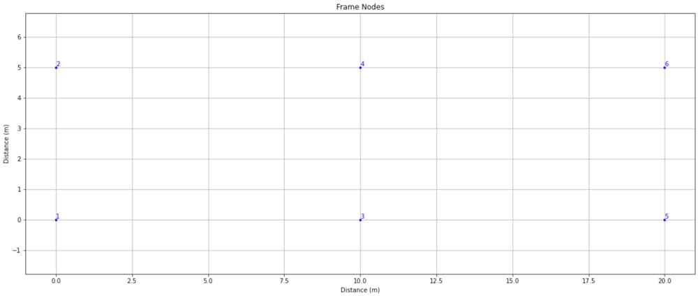
Fig. 6 Plot of newly defined OpenSeesPy model nodes using OpsVis.
We can see that the nodes have been defined, and the ordering of node tags also confirms that our code worked as expected, cycling through each column and defining the base node followed by the eaves node.
Elements
Defining elements for our model requires us to first define a linear geometric transformation that maps member actions and stiffness from the member’s local coordinate system to the global coordinate system. You can read more about this here.
In our analysis, we’re dealing with a planar structure and so we can simply generate a transformation using the default transform; in our case, this would be:
transfType = 'Linear'
transfTag = 1
geomTransf(transfType, transfTag)
We will reference this coordinate transformation by its transfTag (1) later when we define our elements. But before we move on, it’s worth spending a little longer on the geomTransf() method.
There is an optional third argument we could have passed, called vecxz. This will be particularly helpful when modelling 3D structures. By specifying vecxz, we can specify the orientation of each element about its own longitudinal axis.
This is particularly helpful when we have an element that is not axisymmetric and possesses different stiffnesses about its principal axes - think of an I-beam - we would definitely want to specify the axis of orientation since its bending stiffness is radically different about both principal axes.
Ok, so vecxz allows us to specify element orientation - but what is it? It’s the local z-axis of the element, represented in the global X, Y, Z reference frame. So, if we take for granted that the local x-axis of the element is the longitudinal axis and the local-y-axis is perpendicular to this and lies in the plane of the structure, then the local z-axis, according to the right-hand rule is perpendicular to the plane of the structure.
For the elements of our planar structure, we would define vecxz as 0,0,1, since it aligns perfectly with the global Z-axis. Note that this assumes:
- the local x-axis for columns points upwards
- the local x-axis for beams is positive to the right.
Otherwise, vecxz would be 0,0,-1 since the local z-axis would point into the plane instead of out of it as per the global Z-axis.
So, we could have also defined our transform as,
geomTransf(transfType, transfTag,0,0,1)
All of this really becomes relevant when we’re analysing 3D structures - for now, the default transformation is sufficient - with or without specifying vecxz.
With that out of the way, we can define our members using the elasticBeamColumn element, docs ref.
We can take a similar approach to our node definition - cycling through each column and defining it. Then cycling through each beam or rafter and defining it. We’ll start with columns.
#Define columns
for i in range(nBays+1):
    eleTag = i+1
    endBottom = (2*eleTag)-1
    endTop = (2*eleTag)

    #Define element (elementType, elementTag, node_i, node_j, Area, YoungMod, Izz, transfTag)
    element('elasticBeamColumn', eleTag, endBottom, endTop, A, E, Iz, transfTag)
    print(f'Column element with tag {eleTag} defined')
Then rafters.
#Define rafters/beams
for i in range(nBays):
    index = i+1
    eleTag = nBays+1+index
    endLeft = 2*index
    endRight = 2*index + 2

    element('elasticBeamColumn', eleTag, endLeft, endRight, A, E, Iz, transfTag)
    print(f'Rafter/Beam element with tag {eleTag} defined')
In the case of columns and rafters the only semi-tricky thing is working out how to identify the node tag for the nodes at each end of the element.
Visualising our nodes and elements with OpsVis
We can now call our plotStructure() function again to visualise our structure with both nodes and elements added.
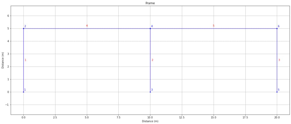
Fig. 7 Plot of newly defined OpenSeesPy model nodes and elements using OpsVis.
Restraints
We define our supports in exactly the same way as for our previous truss analysis - simply by calling the fix() method and passing the relevant node tag and fixity (0 or 1) for each degree of freedom at that node.
We’ll do this in a loop so our code will work for any nBays value.
for i in range(nBays+1):
    index=i+1 #Want iterator to start at 1 nor zero (preference)
    nodeTag = int((2*index)-1) #Base node for this column

    #Pre-append nodeTag to fixity tuple
    nodeFixity = (nodeTag,) + fixity

    #Unpack nodeFixity contents into argument for 'fix' method
    fix(*nodeFixity)
We again call plotStructure() to make sure everything went according to plan. The purple blocks on the column base nodes indicates that our built-in restraints were correctly defined.
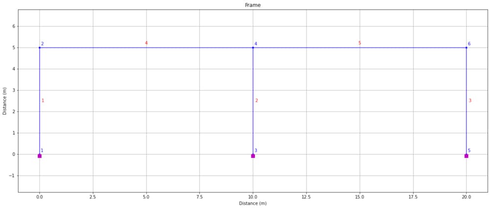
Fig. 8 Plot of newly defined OpenSeesPy model nodes, elements and restraints using OpsVis.
3.4 OpenSeesPy - Load definition
timeSeries and pattern
We start every load definition by first defining a timeSeries and load pattern. These two steps are identical to what we did back in our truss analysis.
# Create TimeSeries with a tag of 1
timeSeries("Constant", 1)

# Create a plain load pattern associated with the TimeSeries (pattern, patternTag, timeseriesTag)
pattern("Plain", 1, 1)
Distributed loads
We apply UDLs (beamUniform) on elements 4 and 5 using the eleLoad method - Doc ref. The arguments to this command are all pretty obvious.
eleLoad('-ele', 4, '-type', '-beamUniform', -10000) # 10kN/m on element 4
eleLoad('-ele', 5, '-type', '-beamUniform', -20000) # 20kN/m on element 5
Nodal/Point loads
The point load at node 2 is applied using a command we’ve seen previously with our truss analysis.
#Point load applied to node 2 in the global X direction
load(2, 200000, 0., 0.)
Plotting loads
OpsVis also has a command for plotting the loads on our structure, plot_loads_2d. We’ll write a new function that combines this method with some of our standard plotting commands.
#Define a new function to plot loads
def plotLoads(title):
    opsv.plot_loads_2d(sfac=True, fig_wi_he=(50,20))
    plt.title(title)
    plt.xlabel('Distance (m)')
    plt.ylabel('Distance (m)')
    plt.grid()
    plt.show()
I noticed a bug with this command - when I executed it initially, the point load at node two didn’t appear in the plot. Executing it a second time seems to solve the problem and get the point load to appear. Note that even when the load wasn’t showing in this command it was still being applied to the structure.
Now we can call both functions to visualise our efforts so far.
plotStructure('Frame')
plotLoads('Frame and Loading')
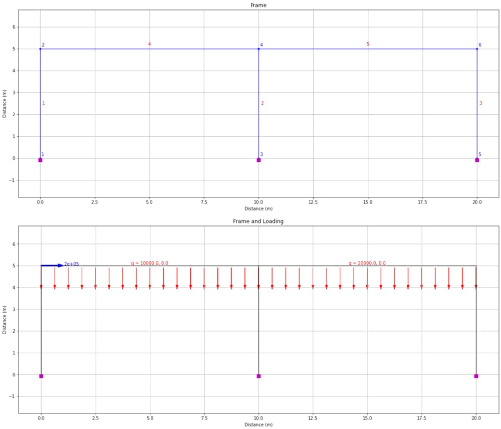
Fig 9. Frame definition (top) and applied loads (bottom) using OpsVis.
3.5 OpenSeesPy - Analysis
Our analysis procedure is more or less a copy of the truss analysis code. I won’t repeat the explanation of each command here, except to note that we’re specifying a different system, BandGeneral and a different constraints option, Transformation.
# Create SOE
system('BandGeneral') # BandGeneral more general solver than 'BandSPD'

# Create DOF number
numberer('RCM')

# Create constraint handler
constraints('Transformation')

# Create integrator
integrator('LoadControl', 1)

# Create algorithm
algorithm('Linear')

# Create analysis object
analysis('Static')

# Perform the analysis (with 1 analysis step)
analyze(1)
BandGeneral as the name suggest and the docs explain, is a more generally applicable equation system than BandSPD which we used previously. With this generality comes a potential efficiency cost - but with the scale of structure we’re working with this isn’t a concern.
In your own analyses - it’s worth experimenting with selecting different equation system options and observing your results and performance.
The constraints command controls how constraint equations are imposed on the system of equations. Again, it’s worth experimenting with Plain and Transformation options to ensure your observed expected behaviour.
4.0 OpenSeesPy Results Visualisation with OpsVis
4.1 Deflection
Now our analysis is complete, we can start extracting some results. Let’s start by examining the deflected shape. We’ll use the plot_defo command from OpsVis and pass some styling parameters so the resulting plot matches, as closely as possible, our original deflected shape plot. As always, you can dig into how best to visually customise your plot by referring to the relevant section of the docs.
s = opsv.plot_defo(fig_wi_he=(50,20),
                   fmt_defo={'color': 'red', 'linestyle': (0, (4, 5)), 'linewidth': 1.5},
                   fmt_undefo={'color': 'green', 'linestyle': 'solid', 'linewidth': 2,},
                  )
plt.title('Deflection')
plt.xlabel('Distance (m)')
plt.ylabel('Distance (m)')
plt.grid()
plt.show()

print(f'The scale factor on deflection is {round(s,2)}')
If we don’t specify a scale factor to apply in the plt_defo command, OpsVis will determine an optimal magnification scale and return it from the command. In this case, our code block prints out…
The scale factor on deflection is 107.35
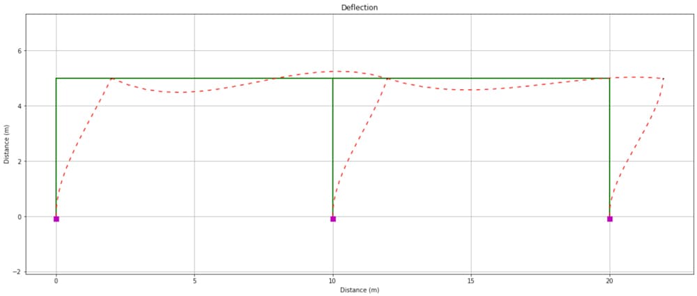
Fig 10. Frame deflected shape determined from OpenSeesPy and visualised using OpsVis.
We can clearly see that the qualitative deflected shape agrees with our original plot from Fig. 2. For a quick quantitative check we can print out the OpenSeesPy model data for node 2 and compare the displacement with that shown on Fig 2.
printModel('-node',2)
This yields…
Node: 2
	Coordinates  : 0 5
	Disps: 0.0186306 -1.96348e-05 -0.00439375
	 unbalanced Load: 200000 0 0
	ID : 6 7 8
Again, we can see that the lateral displacements agree. We could do this for as many nodes as we like - we’ll find that the displacements agree. Note that if you want to print out the complete dataset associated with the model, just use printModel()
At this point we can use the relevant OpsVis commands to generate the bending moment diagram, shear force diagram and axial force diagram. In each case, we’ll see that the OpenSeesPy model output is in agreement with our original model - satisfying our original objective!
4.2 Bending moment diagram
The (colour-customised) bending moment diagram is obtained with the following code. Note that a scale factor, mFac is applied to the diagram to accentuate the bending moments. A corresponding factor will be applied to the shear force and axial force diagrams.
mFac = 5.e-6

opsv.section_force_diagram_2d('M', mFac, fig_wi_he=(50,20),
                             fmt_secforce1={'color': 'green'},
                             fmt_secforce2={'color': 'green'})

plt.title('Bending Moment Diagram')
plt.xlabel('Distance (m)')
plt.ylabel('Distance (m)')
plt.grid()
plt.show()
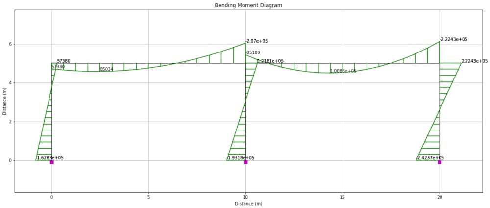
Fig 11. Bending moment diagram determined from OpenSeesPy and visualised using OpsVis.
4.3 Shear force diagram
The shear force diagram is obtained using,
vFac = 15.e-6

opsv.section_force_diagram_2d('V', vFac, fig_wi_he=(50,20),
                             fmt_secforce1={'color': 'red'},
                             fmt_secforce2={'color': 'red'})

plt.title('Shear Force Diagram')
plt.xlabel('Distance (m)')
plt.ylabel('Distance (m)')
plt.grid()
plt.show()
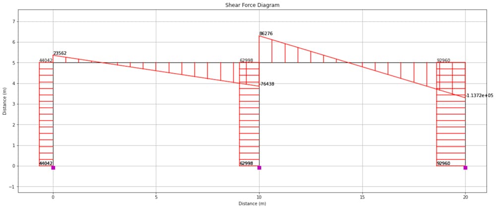
Fig 12. Shear force diagram determined from OpenSeesPy and visualised using OpsVis.
4.4 Axial force diagram
Finally, the axial force diagram is obtained with,
nFac = 10.e-6

opsv.section_force_diagram_2d('N', nFac, fig_wi_he=(50,20))

plt.title('Axial Force Diagram')
plt.xlabel('Distance (m)')
plt.ylabel('Distance (m)')
plt.grid()
plt.show()
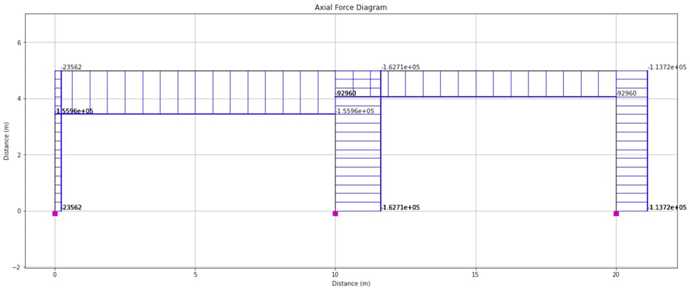
Fig 13. Axial force diagram determined from OpenSeesPy and visualised using OpsVis.
5.0 Testing our parameterisation
Now that our analysis pipeline has been validated, we can play with the parameters we established at the outset to analyse a completely different structure will almost no extra effort! This is where the power of Python scripting and parameterisation, specifically, really comes into focus.
For example, let’s say we have 5 bays instead of two with an eaves height of 10m and a bay width of 12m.
nBays = 5 #Number of bays
h_bay = 10 #(m) #Portal height
w_bay = 12 #(m) #Portal width
Our code will now give us the following annotated structure diagram.
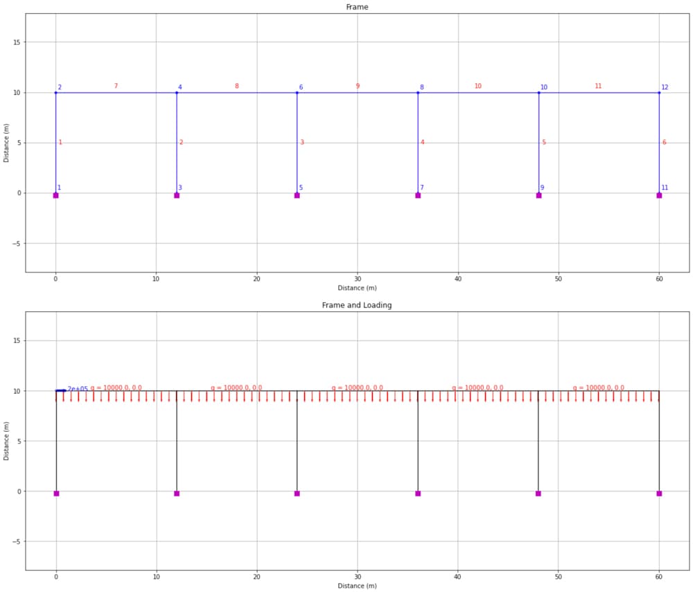
Fig 14. Portal frame structure with 5-bays (top) and applied loading (bottom).
Let’s also imagine we want to apply a uniformly distributed load to all of the rafters. From Fig 14 we can see that the rafters have element tags 7 to 11. So we can apply a 10 kN/m UDL to all elements in one eleLoad command using the -range flag, as follows.
eleLoad('-ele', '-range', 7,11, '-type', '-beamUniform', -10000) # 20kN/m on element 7-11
This will yield the following deflection, bending moment, shear force and axial force diagrams. Note that in each case the scale factor has been tweaked to produce a legible diagram.
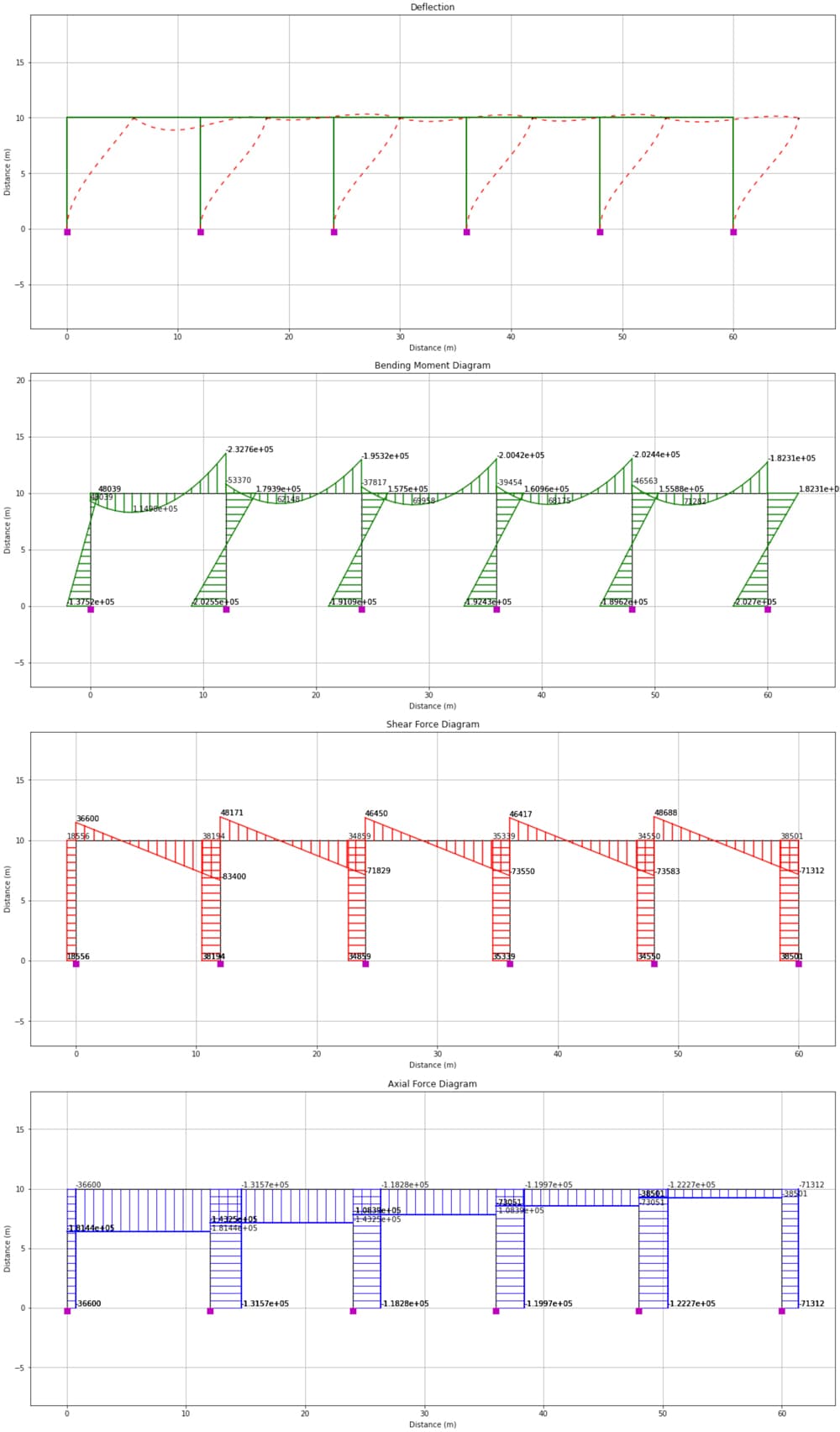
Fig 15. From top to bottom; deflected shape, bending moment diagram, shear force diagram and axial force diagram.
6.0 Conclusion
This brings us to the end of our case study analysis. By now, you should have a good grasp of:
- How to define a 2D frame model using OpenSeesPy (continuous beams would be just as easy!).
- How we can use parameterisation to make our codes more versatile.
- How to define different loads on the structure.
- How to perform a linear elastic structural analysis using OpenSeesPy
- How to quickly produce output diagrams using OpsVis
After working through this tutorial, you’re in a great position to take what you’ve learned, modify it and apply it to your own analyses.
Remember, using a tool like OpenSeesPy, is really only advisable if you understand what it’s doing for you behind the scenes. This is even more true when there’s no graphical user interface to help you flag errors in your implementation. If you don’t understand the theory, it’s much easier to make mistakes!
If you want to understand how the analysis we’ve just completed actually works, from first principles, by writing the code from scratch, take a look at my course, Beam and Frame Analysis using the Direct Stiffness Method in Python.
Beam and Frame Analysis using the Direct Stiffness Method in Python
Build a sophisticated structural analysis software tool that models beams and frames using Python.
After completing this course...
- You’ll understand how to model beam elements that resist axial force, shear forces and bending moments within the Direct Stiffness Method.
- You’ll have your own analysis software that can generate shear force diagrams, bending moment diagrams, deflected shapes and more.
- You’ll understand how to model rotational pins within your structures, inter-nodal distributed loading and realistic flexible supports.
That’s it for this one - more OpenSeesPy on the way soon.
See you in the next one!
Dr Seán Carroll's latest courses.

Featured Tutorials and Guides
If you found this tutorial helpful, you might enjoy some of these other tutorials.
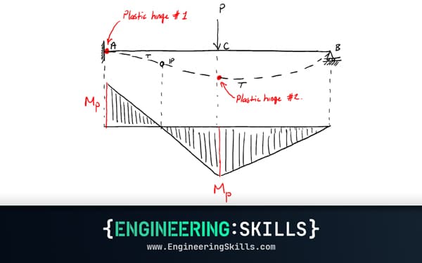
Yielding, Plastic Deformation and Moment Redistribution in Beams (2/2)
Learn how calculate plastic moment capacities and how moment redistribution occurs in a structure

Dr Seán Carroll
![A Structural Modelling and Analysis Addon for Blender [RELEASED]](/_next/image?url=%2Fimages%2Fposts%2Fa-structural-modelling-and-analysis-addon-for-blender%2Fa-structural-modelling-and-analysis-addon-for-blender.jpg&w=1200&q=75)
A Structural Modelling and Analysis Addon for Blender [RELEASED]
You can now download the complete StructureWorks addon!
Dr Seán Carroll