Simulating crowd vibrations using the Duhamel Integral
![[object Object]](/_next/image?url=%2Fimages%2Fauthors%2Fsean_carroll.png&w=256&q=75)
In this Python mini-project, you’ll learn about the Duhamel Integral and how it can be used to simulate the dynamic response of a single degree of freedom system. We’ll discuss how to solve the integral and then write some Python code to implement our solution for any arbitrary loading. In the second half of this project, we’re going to use our Duhamel Integral solver to build a crowd loading simulation. This will allow us to simulate the vibration response of a footbridge to pedestrian traffic.
As usual, this project is accompanied by a complete HD video series. You can access the full playlist for free, by enrolling in the project. In the video series, we’ll walk through the build process line by line. So you can build along with me or if you prefer, just download the finished Python code after you enrol in the project.
I recommend reading through this post (which is a summary of the full project) to get a good overview of the build process and then working through the complete project in more detail.
Simulating Crowd-induced Vibrations using the Duhamel Integral
In this Python project, we build a crowd-induced vibration simulation using the Duhamel Integral in Python
After completing this project...
- You will understand how to use the Duhamel Integral to calculate the dynamic response of SDoF systems
- You will be able to implement the solution using Python in a Jupyter Notebook
- You will understand how this numerical solution can be used to simulate the response due to quasi-random human-induced excitation
- You will be able to build a data visualisation to communicate the output of your simulation
If you’re new to Python, don’t worry – you don’t need to be a Python programmer to complete this project! Complete beginners can work through this project and pick up the programming basics along the way. If you need help getting your coding environment setup, check out this lecture (part of another course but covers what you need to get up and running). So, with all of that out of the way, let’s get into it.
1.0 The Duhamel Integral – Basic Concept
The Duhamel integral is a simple way to simulate the response of a single-degree-of-freedom (SDoF) system to any form of dynamic loading. When the loading is described by a simple mathematical function, we can analytically solve the integral. However, for practical application, this is very often not the case. If the loading is more complex or defined by a time-history of discrete force values, numerical integration can be employed.
We’ll cover the details of how the integration can be handled in both cases. For now, we just need to understand the concept behind the Duhamel integration approach. We can start by considering an impulse. This is simply a force, , that is applied for a very short duration, say . The impulse of the force is defined as the area below the force-time history. So, a unit impulse would have an area of ,
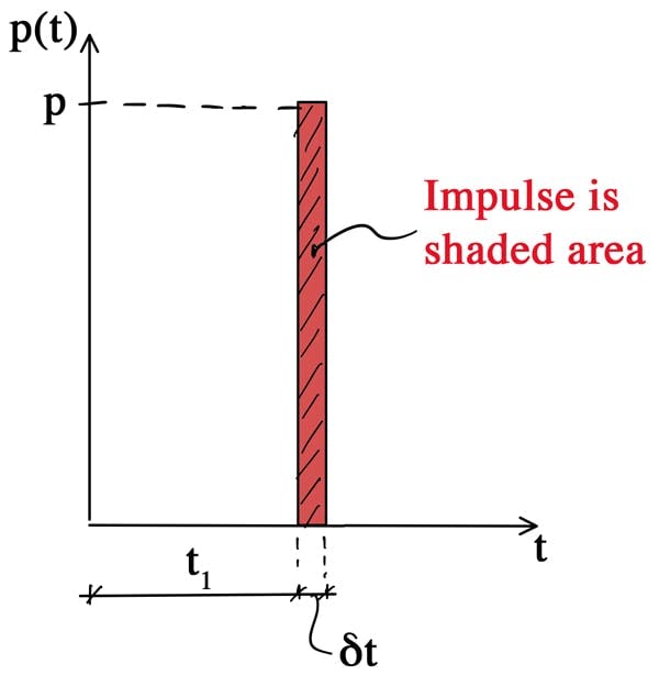
Figure 1. Impulse associated with the force applied for duration
Now, let’s think about applying an impulse to a SDoF system. We’ll see below that we can determine an expression for the resulting free vibration response of the system. Remember, the impulse is a very short duration, high magnitude load. So, it will induce a short duration driven response followed by a decaying (we’ll assume a damped system) free vibration response.
So, how do we use this new information to simulate the response of a SDoF system to general dynamic loading? The trick is to consider the general dynamic loading as a sequence of short duration impulses. Each impulse will induce a free-vibration response. To obtain the overall dynamic response, we simply superimpose the free vibration responses due to each impulse, Fig. 2.
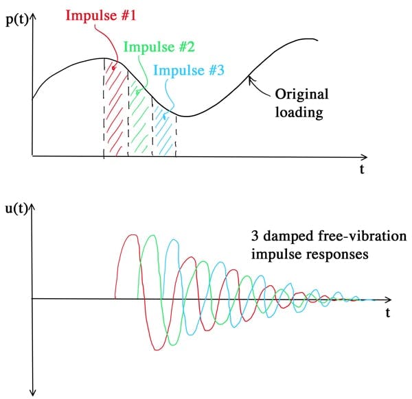
Figure 2. General dynamic loading considered as a sequence of impulses yielding free-vibration responses that can be superimposed to obtain the response to the original dynamic loading.
Hopefully you can see that at a concept level, there’s not much complexity to the Duhamel integral. It’s a very simple but versatile tool. There is one limitation to be aware of. Because we rely on superposition to obtain the overall structural response we must assume the behaviour of the dynamic system is linear. If this is not the case, an alternative solution strategy should be sought, such as direct integration of the equation(s) of motion. We cover this in more detail in my Multi-Degree of Freedom Dynamics course.
Multi-Degree of Freedom Dynamics, Modal Analysis and Seismic Response Simulation in Python
Build the knowledge and tools to decode the dynamic response of real-world structures to real-world loads.
After completing this course...
- You will be able to model the influence of earthquake-induced ground motion.
- You will develop numerical tools to solve the coupled equations of motion for multi-degree of freedom systems.
- You will understand the role of modal decomposition in uncoupling the equations of motion and identifying the underlying dynamic characteristics of MDoF systems.
1.1 Damped Impulse Response
Our next task is to determine an expression for the impulse response of our SDoF system. We start by considering Newton’s second law which states that the rate of change of velocity is directly proportional to the force that causes it, mathematically we have,
Rearranging slightly, we have,
Notice that is actually an impulse; recall from above that the impulse associated with force was the area below the force-time history, . We can see that the impulse induces an instantaneous change in velocity, . Also note that we’ve introduced the time variable , distinct from , to represent the time of application of a specific impulse. This will become clearer when we see both and in the same expression below.
The instantaneous change in velocity, can equally be interpreted as an initial velocity, associated with the application of the impulse,
Now our problem reduces to determining the free vibration response of a SDoF system with non-zero initial velocity at time . We can show that the damped free vibration response of a SDoF system is given by,
where, is the damping ratio, is the angular natural frequency, is the damped natural frequency and is the initial displacement. We cover the derivation of this equation in my Fundamentals of Structural Dynamics course.
Fundamentals of Engineering Structural Dynamics with Python
Leverage fundamental structural dynamics to build your own flexible numerical solutions in Python.
After completing this course...
- You’ll understand how to model dynamic behaviour using spring-mass-damper models and how to simulate free vibration behaviour.
- You’ll be able to model the influence of harmonic loading and how to characterise the transient and steady-state responses.
- You’ll be able to use Python to implement the Piecewise Exact Method to model any form of general dynamic loading.
Now, if we assume the impulse is applied at time , let and let equal to the value in equation 3, we can obtain an expression for the incremental response, due to the impulse applied at time ,
Note that we now have the quantity of time elapsed since the impulse was applied, denoted as . This is why we introduced the time variable originally. We’re not quite finished; remember that to get the total response of the system at time , we need to sum up or superimpose the influence of all of the impulses applied, up to this point in time. We can do this by integrating both sides of equation 5,
This expression is what we refer to as Duhamel’s integral – the next step is to solve it.
2.0 Analytical Solution
As we said at the outset, there are two approaches to solving the Duhamel integral (or any integration really), analytical solution and numerical solution. By far the most practically useful method is numerical solution. Most of the interesting problems, from an engineering perspective, require numerical solution. Although a numerical solution will always be an approximation, any error introduced usually pales into insignificance when compared against other uncertainties bakes into our modelling.
Numerical solution comes with the huge advantages of simplicity and versatility. I’ve always been more of a programmer than a mathematician so I may be biased. Having said all of this, we will demonstrate an analytical solution first for completeness; even then we’ll use Python to do the hard work.
Ramp Loading
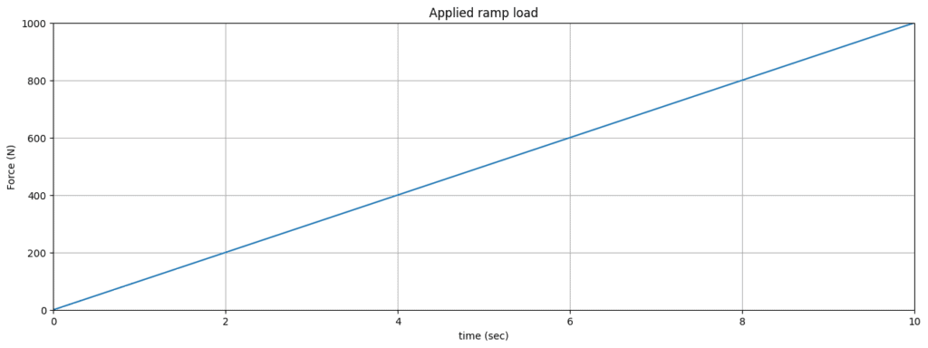
Consider a load that increases linearly from zero to a magnitude of between and . We can represent the loading with a simple mathematical expression,
The fact that the applied loading can be captured with such a simple expression is the first clue that we might be able to solve this analytically. Assigning some arbitrary values to and we can generate a plot of the loading.
# DEPENDENCIES and DEFAULTS
import math #.....................................Math functionality
import numpy as np #..............................Numpy for working with arrays
import matplotlib.pyplot as plt #.................Plotting functionality

P0 = 1000 #(N) Max load (arbitrary value for visualisation only)
t1 = 10 #(sec) Rise time (arbitrary value for visualisation only)
delT = 0.1 #(sec) Time-step
t = np.arange(0, t1+delT, delT) #Time vector
p = P0*t/t1#Force vector

#Set up figure and axes
fig = plt.figure()
axes = fig.add_axes([0.1,0.1,2,1])
axes.plot(t,p)

#Housekeeping
axes.set_xlabel('time (sec)')
axes.set_ylabel('Force (N)')
axes.set_title('Applied ramp load')
axes.set_xlim([0,t1])
axes.set_ylim([0,P0])
plt.grid()
plt.show()
Next, we can insert our expression for the applied loading directly into the Duhamel integral expression.
In this case, we are only considering the response of the system during the application of the ramp load and not the free vibration that would follow. As such, damping will not have an appreciable influence on the response. We can therefore simplify the task by considering an undamped system. As a result, our expression reduces to,
Now we need to integrate this expression, for this we’ll use SymPy.
import sympy as sym #Import SymPy
sym.init_printing() #So we print nicely formatted equations

#Define some symbols
m = sym.Symbol('m')
w = sym.Symbol('w')
P0 = sym.Symbol('P0')
t1 = sym.Symbol('t1')
tau = sym.Symbol('tau')
t = sym.Symbol('t')

#Construct the function to integrate
f = tau * sym.sin(w*t-w*tau)

# Use SymPy to get the definite itegral with respect to tau between 0 and t

defInt = sym.integrate(f,(tau,0,t))

print('SymPy generated the following expression for the definite integral:')
sym.simplify(defInt) #Attempt to siplify the definite integral
Combining the output from SymPy with the remaining elements from equation 9 yields,
We can further rearrange this,
To complete the picture, we can plot the response. When plotting we will normalise the time axis by the rise time and normalise the displacement axis by the maximum static displacement, .
#Redefine constants following symbolic math operations
P0 = 1000 #(N) Max load
t1 = 10 #(sec) Rise time
delT = 0.1 #(sec) Time-step
t = np.arange(0, t1+delT, delT) #Time vector
We’ll perform the response calculation for a range of different SDoF systems with the same mass but different stiffness, yielding a range of natural frequencies. For each system, we’ll specify the period of the system as a proportion of the rise time of the load.
m=20 #Mass of the system
periodRange = [0.3,0.4,0.5] #Range of system periods as a propertion of rise time

#Initialise a figrue to plot onto
fig = plt.figure()
axes = fig.add_axes([0.1,0.1,2,1])

for pr in periodRange:
  T = pr*t1
  wn = 2*math.pi/T
  k=m*wn**2
  u = (P0/k)*((t/t1)-((np.sin(wn*t))/(wn*t1)))
  axes.plot(t/t1,u/(P0/k), label=f"T = {pr}t1")

#Housekeeping
axes.set_xlabel('t/t1')
axes.set_ylabel('Displacement ratio')
axes.set_title('SDoF system response to ramp loading')
axes.legend(loc='upper left')
axes.set_xlim([0,1])
plt.grid()
plt.show()
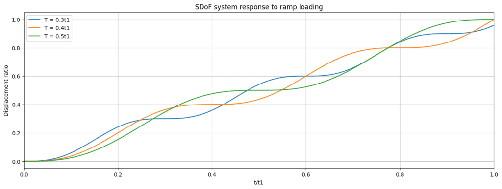
This example is a relatively trivial case but it demonstrates the analytical integration route to solving the Duhamel integral. As I mentioned, you’re not likely to deploy analytical integration too often, so we’ll leave this method behind and focus on numerical integration from here on.
3.0 Numerical solution
From what we’ve seen so far, solving the Duhamel integral analytically is certainly possible, but as we’ve already mentioned, real-life engineering is messy and often we can’t neatly describe our applied loading in a mathematical function. This is where the numerical solution strategy comes in. In this section we’ll build a function that numerically solves the Duhamel integral for any arbitrary loading we pass into the function. We’ll start by restating the Duhamel integral for a damped system,
We can separate out the time variables with the help of a trigonometric identity,
Since we’re integrating with respect to we can restructure our expression to isolate the terms requiring numerical integration,
where,
and now represent two integrals that we can numerically evaluate. We’ll use the trapezoidal rule here; we’ve covered this in some detail in our beam deflection calculator project so we’ll only briefly summarise the key points here.
If we consider the integrand (of or ) as a simple function, , we could plot this function on a plane. We know that the integration is simply the area bounded by the function and the horizontal axis. Using the trapezoidal rule we can approximate this as,
Now all that remains is to write a function to cycle through the time history computing the numerical integrations in equations 15 and 16 and then compute the response using equation 14.
3.1 Implementing the numerical solution
We’ll package all of our code into a function that accepts a time and force vector. This way we can easily reuse the Duhamel integral function from this file and deploy it elsewhere down the road. Let’s start by defining SDoF system parameters; mass , damping ratio and natural frequency/angular natural frequency . We can also define the damped natural frequency, .
m = 1000 #(kg) Mass
xi = 0.05 # Damping ratio
f = 1.5 #(Hz) Natural frequency
wn = 2*math.pi*f #(rads/s) Angular natural frequency
wd = wn*math.sqrt(1-xi**2) #(rads/s) Damped angular natural frequency
For the purposes of demonstration here we’ll define a harmonic forcing function. This will make it easier to validate our Duhamel integral function against a closed-form solution. First, we can define a time vector in the usual way.
tMax = 20 #(s) Max time
delT = 0.01 #(s) Time-step
time = np.arange(0, tMax+delT, delT) #Time vector

f_Force = 1 #(Hz) Forcing frequency
wf = 2*math.pi*f_Force #(rads/s) Angular forcing frequency
P=100 #(N) Force amplitude
force = P*np.sin(wf*time) #Force vector
The function we write next will accept the time and force vectors as arguments. We’ll rely on the fact that all of the system parameters a defined globally so we won’t bother explicitly passing them into the function. We basically need to cycle through the time record and compute the area of the trapezoid and add this to a cumulative sum of areas as we move along the time axis. In this way, we can calculate appropriate values for and (equations 15 and 16) at each time-step. Then, we can calculate the actual response for each time-step using equation 14. If I’ve lost you with the trapezoidal method of numerical integration, go back to the beam deflection tutorial I referenced earlier. I walk through this technique from scratch there.
def Duhamel(T, F):
  #Initialise a container of zeros to hold the displacement values
  U = np.zeros(len(T))

  #Initialise values for the cumulative sum used to calculate A and B at each time-step
  ACum*i=0
  BCum*i=0

  #Cycle through the time vector and evaluate the response at each time point
  for i, t in enumerate(T):
    #Only start calculating on the second iteration (need two values for trapezoidal area calculation)
    if i>0:

      #Calculate A[i] - equation 4
      y_i = math.e**(xi*wn*T[i]) * F[i] * math.cos(wd*T[i]) #Value of integrand at current time-step
      y*im1 = math.e**(xi*wn*T[i-1]) * F[i-1] * math.cos(wd*T[i-1]) #Value of integrand at previous time-step
      Area*i = 0.5*delT*(y_i+y_im1) #Area of trapezoid
      ACum_i += Area_i #Cumulative area from t=0 to current time
      A_i = (1/(m*wd))*ACum_i #Value of A for the current time-step

      #Calculate B[i] - equation 5 (same notes as for A above)
      y_i = math.e**(xi*wn*T[i]) * F[i] * math.sin(wd*T[i])
      y*im1 = math.e**(xi*wn*T[i-1]) * F[i-1] * math.sin(wd*T[i-1])
      Area_i = 0.5*delT*(y_i+y_im1)
      BCum_i += Area_i
      B_i = (1/(m*wd))*BCum_i

      #Calculate the response - equation 3
      U[i] = A_i*math.e**(-xi*wn*T[i])*math.sin(wd*T[i]) - B_i * math.e**(-xi*wn*T[i])*math.cos(wd*T[i])

  return U
Now that we have the function defined we just need to call it and assign the output to a variable for plotting.
response = Duhamel(time, force) #Response calculated using the Duhamel integral function

#Initialise a fig to plot onto
fig = plt.figure()
axes = fig.add_axes([0.1,0.1,2,1])
axes.plot(time,response)

#Housekeeping
axes.set_xlabel('time (s)')
axes.set_ylabel('Disp (m)')
axes.set_title('SDoF system response to harmonic loading')
axes.set_xlim([0,tMax])plt.grid()plt.show()
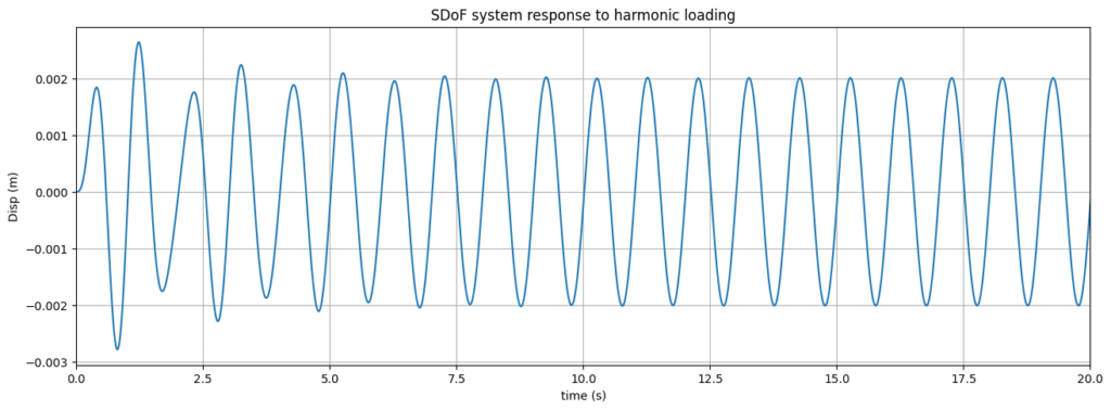
We can see above that the response contains a transient component that dissipates due to damping leaving a steady-state response which is exactly what we would expect from the harmonic excitation of a SDoF system.
4.0 Validating our numerical solution
Now we’ll confirm the validity of our Duhamel function by comparing the calculated response with the closed-form (analytical) solution for harmonic loading of a SDoF system. We could plot the complete closed-form response including the transient and steady-state components but for our validation exercise it will be sufficient to only plot the steady-state response, given by,
If you’ve studied fundamental structural dynamics, you will recognise this as the dimensionless form of the steady-state response equation – if this is completely unfamiliar and you don’t like equations dropping out of thin air, go here.
#Steady-state response
beta = wf/wd #Frequency ratio
k=m*wd**2 #(N/m) Stiffness

#Break equation into two for convenience
O = (P/k)*(1/((1-beta**2)**2 + (2*xi*beta)**2))
response_cf = O*((1-beta**2)*np.sin(wf*time) - 2*xi*beta*np.cos(wf*time))
fig = plt.figure()
axes = fig.add_axes([0.1,0.1,2,1])
axes.plot(time,response, '-', label='Duhamel')
axes.plot(time,response_cf,'-',label='Closed-form')

#Housekeeping
axes.set_xlabel('time (s)')
axes.set_ylabel('Disp (m)')
axes.set_title('SDoF system response to harmonic loading')
axes.legend(loc='lower right')
axes.set_xlim([0,tMax])
plt.grid()
plt.show()
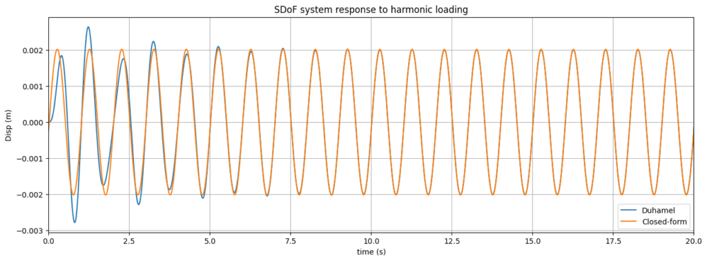
We can see that both solutions agree once the transient response has decayed away. This gives us confidence in the Duhamel integral code we’ve written. This is quite a powerful tool we have at our disposal now. Although we only used it to calculate the response due to harmonic loading, we can feed it any forcing function and it will return the SDoF system response.
So, in the next phase of this project, we’ll use our Duhamel integral function to do something a little more interesting. We’re going to estimate the vertical vibration response of a footbridge to pedestrian traffic. Although, we’ll focus on a simply-supported footbridge, the same principles can be applied to crowd-induced vibration of any structure, although there are some specific caveats we’ll discuss along the way.
5.0 An introduction to dynamic crowd loading
Volumes of research has been produced on the topic of human-induced vibration and in particular crowd-induced vibration. Research in this area has intensified in the last 20 years as structures, in particular floor plates, have become lighter and more slender. This has resulted in unacceptably large occupant-induced vibrations being observed in service more frequently. There is now a much greater understanding among engineers and other procurement stakeholders about the need to carefully asses vibration serviceability at design stage.
For the purposes of this analysis project, when we say human-induced vibration, we’re referring to the vibration induced by a single pedestrian as they walk. Crowd-induced vibration will refer to the response induced by multiple people simultaneously walking across a structure.
Human-induced vibration is a complex and fascinating dynamic problem because it involves interaction between the structure and the occupying pedestrian, both of which are dynamic systems. The problem gets even more interesting (and complex) when we start to introduce interaction between pedestrians and try to capture the tendency for a pedestrian to be influenced by the behaviour of those around them. We won’t attempt to dive in to the detail too much here but we do need some understanding of the problem before we start coding.
In addition to dividing the problem into human-induced and crowd-induced vibration, we can further divide the problem into one that considers vertical vibration and one that considers lateral vibration. Human locomotion response and balance behaviour is very different in each case. We’ll focus here on vertical vibration and leave the juicy problem of lateral human-structure interaction and synchronisation for another day!
Footfall force modelling 101
In the simplest of terms, when a person walks across a structure, in our case a linear footbridge, they will apply a vertical footfall force or ground reaction force (GRF) with each footstep. We can crudely model this GRF using a sine function, or more specifically a series of sine functions representing the harmonic components of the GRF. This assumes that the GRF is perfectly periodic which is itself a simplification but we can live with it. So, the GRF can be represented as the static weight of the pedestrian, , added to a Fourier series representing the dynamic component of loading,
where, is the Fourier coefficient (also knows as a Dynamic Load Factor), is the phase of the harmonic and is the pacing frequency. We will only concern ourselves with the fundamental harmonic, i.e. that component of the GRF at the pacing frequency. We’ll ignore the higher integer harmonics in this example, but these may be significant, depending on the dynamic characteristics of the structure in question.
In order to model the GRF we need to know the Fourier coefficient of the fundamental harmonic. Again there has been a lot of research work on this over the years but we’ll use an early relationship proposed by Kerr [1] that relates the to the pacing frequency, ,
This relationship is valid for pacing frequencies between and . Now, this raises the question of what should the pacing frequency be? For this we’ll rely on a relationship presented by Bruno and Venuti [2] that was developed from the earlier work of Bertram & Ruinne [3],
where is the walking velocity. Of course now we’re presented with the task of working out what a sensible walking velocity should be. Here we’ll rely on work by Pachi and Ji [4] who observed that walking velocities in a sample of pedestrians were normally distributed with a mean value of and a standard deviation of .
An import feature in the modelling of crowd-induced vibration is the flow behaviour of the pedestrian crowd and their evolving distribution across the structure. As a pedestrian crowd becomes more dense, walking velocities are reduced due to congestion. However in this analysis, we’ll ignore all traffic effects due to interaction between pedestrians. This is a reasonable assumption for uncongested crowds where it’s reasonable to expect that an individual’s desired walking velocity won’t be constrained by neighbouring pedestrians.
We’re now at a point where we can approximate the GRF imparted by a pedestrian with a mass of walking with a velocity of in a straight line. If we assume the pedestrian walks across a long footbridge, it will take then seconds to cross the bridge. This gives us the duration of load application.
L = 60 #(m) Bridge span
vp = 1.3 #(m/s) Pedestrian walking velocity
tMax = L/vp #(s) Crossing time
m = 80 #(kg) Pedestrian mass
G = 9.81*m #(N) Static weight of pedestrian

fv = 0.35*vp**3 - 1.59*vp**2 + 2.93*vp #(Hz) Pacing frequency
DLF = 0.41*(fv-0.95) #Dynamic load factor

print(f"- The DLF = {round(DLF,3)} and the pacing frequency is {round(fv,2)} Hz ({round(fv,2)} steps per second)")
print(f"- Duration of a single step is {round(1/fv,2)} seconds")
-> The DLF = 0.386 and the pacing frequency is 1.89 Hz (1.89 steps per second) -> Duration of a single step is 0.53 seconds
Now we can define the time vector and plot the GRF. Note that we’re only interested in the positive value of the GRF as the footfall force never acts to pull the walking surface upwards! This means that a single sine wave actually models 2 footsteps – this is why the frequency is divided by 2 in the code below.
delT = 0.005 #(s) Time-step
time = np.arange(0, tMax+delT, delT) #Time vector
Fv = G + abs(G*DLF*np.sin(2*math.pi*(fv/2)*time)) #Static + Dynamic GRF

fig = plt.figure()
axes = fig.add_axes([0.1,0.1,2,1])
axes.plot(time,Fv, '-', label='GRF')

#Housekeeping
axes.set_xlabel('time (s)')
axes.set_ylabel('Force (N)')
axes.set_title('Vertical ground reaction force')
axes.legend(loc='lower right')
axes.set_xlim([0,5])
plt.grid()
plt.show()
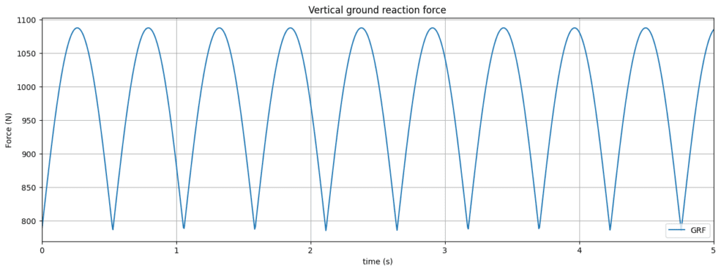
Each of the half-sine peaks represents the force generated by one foot hitting the surface. Remember, a more rigorous model would need to consider the influence of varying walking speed. Even when we make the assumption of constant walking speed, the GRF is not a perfectly periodic function so there is some approximation involved in representing it as a Fourier series.
Furthermore, we’re only representing the fundamental harmonic component here – an actual recorded GRF resembles a square wave more than a half-sine wave. Nevertheless, this will still give us a reasonably realistic first approximation of human-induced vibration response when we apply it to a structure.
It’s also worth pointing out that in our modelling we’re going to assume that there is no human-structure interaction. This is generally a bigger problem for lateral oscillations, due to the fact that humans tend to exhibit higher sensitivity to lateral support motion versus vertical motion. This is likely a result of our bi-pedal nature and inherent instability in the lateral direction. So, just to be clear, we’re assuming the vertical bridge motion does not influence the pedestrians behaviour (and their GRF) in any way.
The bridge/beam structure
Now we can turn our attention to the bridge structure. We’ll keep things simple here and assume that our bridge can be modelled as a simply supported beam. This means that the modal properties are easily obtained. In particular we’re interested in the mode shapes, which can be obtained from,
where is the mode number and is the longitudinal coordinate along the bridge/beam. For a deeper dive into modal analysis, refer to my Multi-Degree of Freedom Dynamics course. We’re going to assume that the fundamental vertical mode of the bridge has a frequency of . This is sufficiently close to the average pacing frequency that if this were a real bridge we would be concerned that unacceptable vibrations may be observed in service.
We’ll assume that the bridge has a damping ratio of and that the mass per unit length, is . We’re going to make another simplifying assumption here; we’ll assume that the mass of pedestrians on the bridge has no influence on the modal mass of the dynamic system being simulated. Our justification here is that the mass of pedestrians is insignificant compared to the mass of the bridge. If this were not the case we could consider modifying the modal mass to reflect the evolving distribution of pedestrians on the bridge. I published a paper [5] on this some time ago that you can read if you want to explore this further. Thanks to this simplification, the modal mass, remains constant and can be calculated from the expression,
So, for the first mode, the modal mass is simply half the actual mass of the structure.
6.0 Dynamic analysis: Bridge + 1 pedestrian
Since we’re assuming that the bridge has only one modal frequency in the range of interest, we only need to simulate a single vibration mode which makes the Duhamel integral an ideal solution technique. Conveniently for us and through the magic of modal analysis, this means that the dynamic analysis of the bridge reduces to simulating the response of a SDoF system. If we needed to simulate the combined response of multiple modes, this is easily done through modal superposition.
Our first task is to turn our GRF, , into a modal force, . This simply means multiplying it by the unity-normalised mode shape value at the pedestrian’s location, ,
Since our pedestrian is walking with a constant velocity, we can easily determine their position, , as a function of time. From here we can determine the value of the mode shape as a function of time and directly multiply this by the GRF calculated earlier to obtain the modal load applied to the SDoF modal model as a function of time.
xp = vp*time #Pedestrian position as a function of time
phi = np.sin(math.pi*xp/L) #Mode shape at pedestrian's location
Fn = Fv*phi #Modal force experienced by SDoF system
At this point it’s helpful to visualise the modal force. Remember, this is the force applied to the first bridge/beam mode with a half-sine mode shape. We can think of this force as the influence of the GRF on mode one which is at a maximum at the centre-span position.
fig = plt.figure()
axes = fig.add_axes([0.1,0.1,2,1])
axes.plot(time,Fn, '-', label='Modal load')

#Housekeeping
axes.set_xlabel('time (s)')
axes.set_ylabel('Force (N)')
axes.set_title('Modal Force')
axes.set_xlim([0,tMax])
plt.grid()
plt.show()
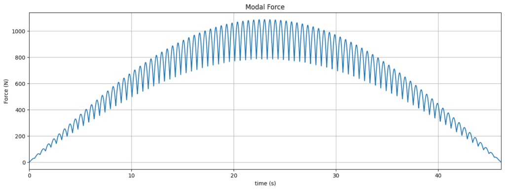
We can clearly see that the dynamic influence of the pedestrian’s GRF is increasing as they move towards the centre of the bridge and diminishing thereafter. Now it’s just a matter of providing this force along with the time vector directly into our Duhamel function. Since our function relies on globally defined variables, we need to be careful to redefine these for our bridge before calling the function.
M = 2000 #(kg/m) Mass per unit length]
m = 0.5*M*L #(kg) Modal mass of mode 1
xi = 0.025 #Damping ratio
fn = 2.5 #(Hz) Bridge modal frequency
wn = 2*math.pi*fn #(rads/s) Angular modal frequency
wd = wn*math.sqrt(1-xi**2) #(rads/s) Damped angular modal frequency
response = Duhamel(time, Fn) #Response calculated using the Duhamel integral function
fig = plt.figure()
axes = fig.add_axes([0.1,0.1,2,1])
axes.plot(time,-response, '-')

#Housekeeping
axes.set_xlabel('time (s)')
axes.set_ylabel('Disp (m)')
axes.set_title('Modal response (static+dynamic)')
axes.set_xlim([0,tMax])
plt.grid()
plt.show()
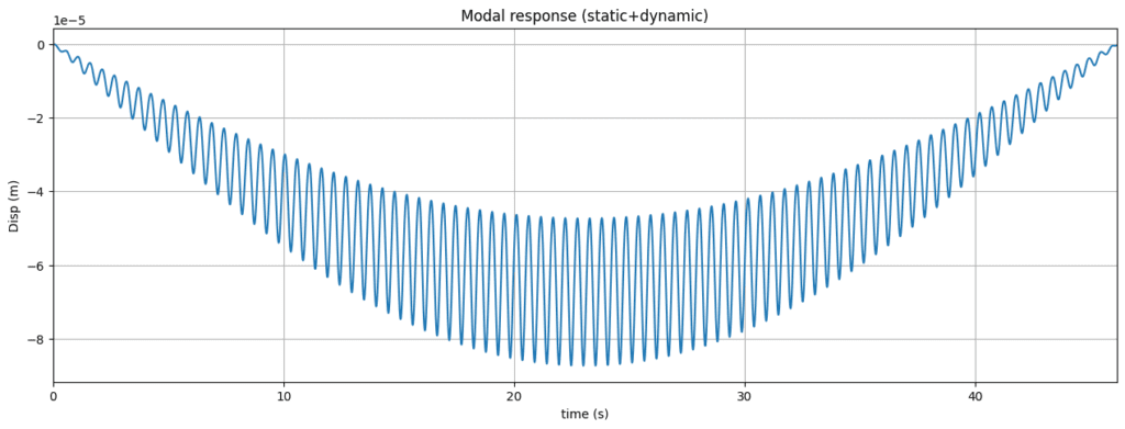
After plotting the modal response we can see the oscillation behaviour superimposed on top of the static deflection. We can visualise this more clearly if we separate out the static and dynamic components of the GRF and simulate their influence separately.
Fn_static = G*phi #Static component of GRF
Fn_dynamic = abs(G*DLF*np.sin(2*math.pi*(fv/2)*time))*phi #Dynamic component of GRF

response_static = Duhamel(time, Fn_static) #Response due to constant magnitude moving load
response_dynanmic = Duhamel(time, Fn_dynamic) #Response due to footsteps (with static load component removed)
fig, axes = plt.subplots(figsize=(14,10),nrows=2,ncols=1)
axes[0].plot(time,-response_dynanmic, '-', label='Dynamic')
axes[0].plot(time,-response_static, 'r-', label='Static')
axes[0].set_xlabel('time (s)')axes[0].set_ylabel('Disp (m)')
axes[0].set_title('Modal response (separate components)')
axes[0].legend(loc='lower right')
axes[0].set_xlim([0,tMax])
axes[0].grid()

axes[1].plot(time,-response, '-', label='Combined')
axes[1].set_xlabel('time (s)')
axes[1].set_ylabel('Disp (m)')
axes[1].set_title('Modal response (combined)')
axes[1].legend(loc='lower right')
axes[1].set_xlim([0,tMax])
axes[1].grid()

plt.show()
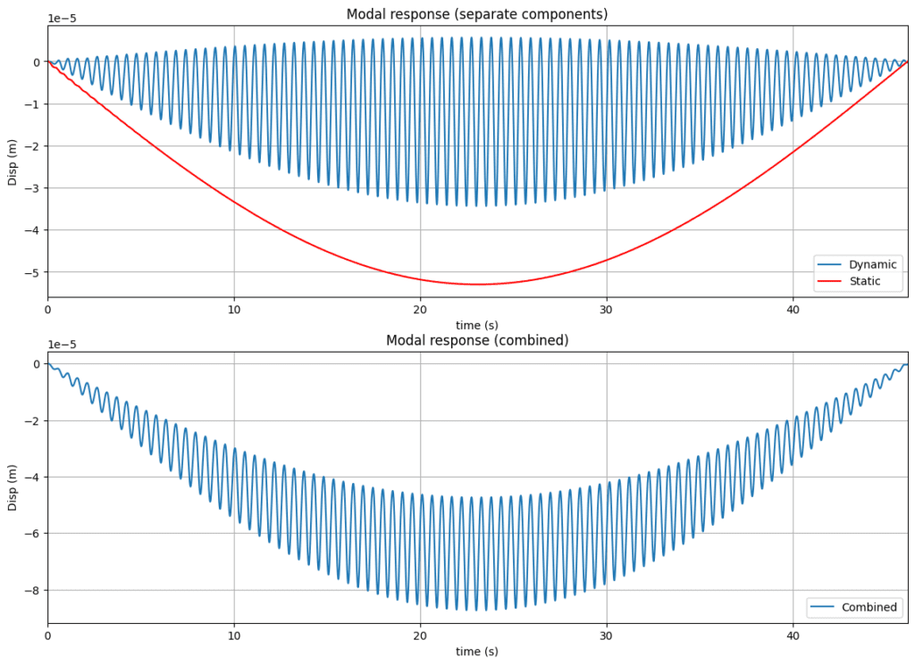
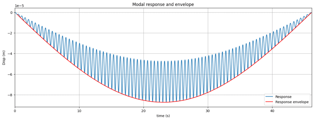
It will help us to more clearly visualise the response if we write a quick function to plot the displacement envelope. This will be particularly helpful later on when our response is derived from the influence of many pedestrians walking simultaneously. We’ll do this by cycling through the displacement record and extracting the oscillation peaks. A peak will be identified when the slope of the displacement changes sign from positive to negative.
This won’t be a perfect strategy as it will also identify ‘minor’ peaks due to frequencies other than the dominant oscillation frequency but it will be close enough for visualisation purposes. Again, we’ll package the code into a function that can be easily called multiple times.
def Peaks(disp, time):
  #Initialise containers to hold peaks and their times
  peaks = np.empty([1,0])
  times = np.empty([1,0])

  #Calculate slopes for each data point
  slopes = np.zeros(len(disp))
  for i, u in enumerate(disp):
    if(i<len(disp)-1):
      slopes[i] = disp[i+1]-disp[i]

  #Cycle through all slopes and pick out peaks
  for i, s in enumerate(slopes):
    if (i<len(slopes)-1):
      if(slopes[i+1]<0 and slopes[i]>0):
        peaks = np.append(peaks,disp[i])
        times = np.append(times,time[i])

  return [peaks, times]
peaks, times = Peaks(response,time)
Now we can plot the response again but also plot an envelope line that spans between oscillation peaks.
fig = plt.figure()
axes = fig.add_axes([0.1,0.1,2,1])
axes.plot(time,-response, '-', label='Response')
axes.plot(times,-peaks,'r-', label='Response envelope')

#Housekeeping
axes.set_xlabel('time (s)')
axes.set_ylabel('Disp (m)')
axes.set_title('Modal response and envelope')
axes.legend(loc='lower right')
axes.set_xlim([0,tMax])
plt.grid()
plt.show()
Complete the final two parts of this project by enrolling for free
Now that we can simulate the mid-span response induced by a single pedestrian as they cross the bridge, we’re ready to expand our simulation to consider a pedestrian crowd consisting of pedestrians. To follow the final two parts of this project,
- 7.0 Dynamic analysis: Bridge + N pedestrian crowd
- 8.0 Animating bridge response & traffic flow
enrol in the accompanying Python project for free. After you enrol you can also watch the complete video walkthrough of the project and download the complete code.
If you want to take a deeper dive into structural dynamics, check out the Structural Dynamics course bundle. This will give you a clear roadmap to mastering structural dynamics and implementing what you know with Python.
[1] S.C. Kerr, Human Induced Loading on Staircases, Ph.D. Thesis, University College London, Mechanical Engineering Department, London, UK, 1998.
[2] F. Bruno, L.and Venuti. Crowd-structure interaction in footbridges: Modelling, application to a real case-study and sensitivity analyses. Journal of Sound and Vibration, 323:475–493, 2009.
[3] J. E. A. Bertram and A. Ruina. Multiple walking speed-frequency relations are predicted by constrained optimization. Journal of Theoretical Biology, 209:445–453, 2001.
[4] A. Pachi and T. Ji. Frequency and velocity of people walking. The Structural Engineer, 83:36–40, 2005.
[5] S.P. Carroll, J.S. Owen, M.F.M. Hussein. Modelling crowd-bridge dynamic interaction with a discretely defined crowd. The Journal of Sound and Vibration, 331:2685-2709, 2012
Dr Seán Carroll's latest courses.


Featured Tutorials and Guides
If you found this tutorial helpful, you might enjoy some of these other tutorials.
Understanding Tresca and von Mises Elastic Failure Theories
Go from the fundamentals of elastic failure theory to implementing section analysis in Python using sectionproperties

Julian Haudek


