An Introduction to OpenSees and OpenSeesPy for 2D Truss Analysis

1.0 Introduction

OpenSees, and by extension OpenSeesPy can be tricky to get started with. The learning curve is relatively steep, but there is a huge amount of functionality packed into the library, so it’s worth persevering with.

I think the difficulty stems from the fact that the official documentation is really quite limited - so this tutorial will hopefully serve as a helpful entry point into the library for anyone completely new to OpenSeesPy. We’re only going to scratch the surface of OpenSeesPy in this tutorial - I plan to write more on this in the future - but for now, this tutorial will be enough to get you up and running and whet your appetite to explore further!

So, what better way to get our feet wet than with a simple example. We’ll expand the original tutorial example from the OpenSeesPy docs and re-analyse a sample structure from my course, The Direct Stiffness Method for Truss Analysis with Python.

In that course, we build a complete analysis code for 2D trusses using the Direct Stiffness Method. As an engineer, it’s obviously important to understand how to implement this analysis from first principles. Having said that, plugging into existing libraries can also be incredibly useful - this is where OpenSeesPy (and this tutorial) comes in.

2.0 A brief history of OpenSees

2.1 Origins of OpenSees

OpenSees is short for Open System for Earthquake Engineering Simulation. It is a software framework originally developed in the late 90’s by Frank McKenna for simulating the seismic response of structures (check out this short video for a brief overview by Frank).

OpenSees was originally developed at the Pacific Earthquake Engineering Research Center (PEER) located at the University of California, Berkeley. OpenSees has now evolved into a robust, multi-purpose simulation platform used by engineers and researchers worldwide.

Originally tailored for earthquake engineering, the capabilities of OpenSees have expanded over the years to encompass a broader range of structural and geotechnical analysis and design.

2.2 OpenSees Today

Today, it’s used in a diverse range of areas, such as performance-based design, collapse assessment, soil-structure interaction, and retrofitting studies, among others. OpenSees excels at handling complex material behaviour, intricate geometric configurations, and advanced analysis procedures.

There is no graphical user interface (GUI), as a result, you’re likely to find OpenSees used more extensively in the world of engineering research with commercial GUI-based packages used in industry. However, if you have a foot in both camps or are comfortable coding, OpenSees is a real hidden gem.

As the name suggests, OpenSees is open-source software. This has been instrumental in its development and proliferation over the last 25 years. Being open-source means that users and contributors from around the globe can access, use, modify, and distribute the software freely. The only caveat to this is that if you intend to sell software that uses OpenSees behind the scenes, you must obtain a license from the University of California.

This collaborative environment has led to ongoing enhancement of its features and capabilities, driven by a community of users and developers committed to advancing the field of earthquake engineering. The open-source model also ensures transparency and reliability, as the code is open for scrutiny, verification, and improvement by the global engineering community.

2.3 OpenSeesPy (the Python version)

So far, all we’ve said relates to OpenSees, the original library, written in C, C++ and Fortran. with user interaction performed using the Tcl (pronounced ‘tickle’) programming language.

The introduction of OpenSeesPy, a Python library for OpenSees, marked a significant milestone in making the framework more accessible. OpenSeesPy opens the door for a much broader audience, particularly as Python has become the preferred language for data analysis, visualisation, and computational scripting within the engineering community.

OpenSeesPy effectively bridges the gap between advanced engineering simulations and the expansive Python ecosystem. It allows engineers and researchers to define models in OpenSees using Python scripting, which is often more intuitive and less steep of a learning curve than the original Tcl scripting language used by OpenSees.

We can also leverage various Python libraries for tasks such as numerical analysis with NumPy and Pandas and data visualisation with Matplotlib or Plotly. As you’ll see in this tutorial, we can also do all of this within the Jupyter Notebook development environment - which is my preferred way to play with Python!

So, now that you have a little more context and background on OpenSees/OpenSeesPy, let’s roll up our sleeves and get stuck into some modelling!

3.0 Analysis Case Study

For our case study structure, we’ll return to an old reliable we’ve used across several tutorials in the past - the inverted bowstring truss from lecture 53 of The Direct Stiffness Method for Truss Analysis with Python course.

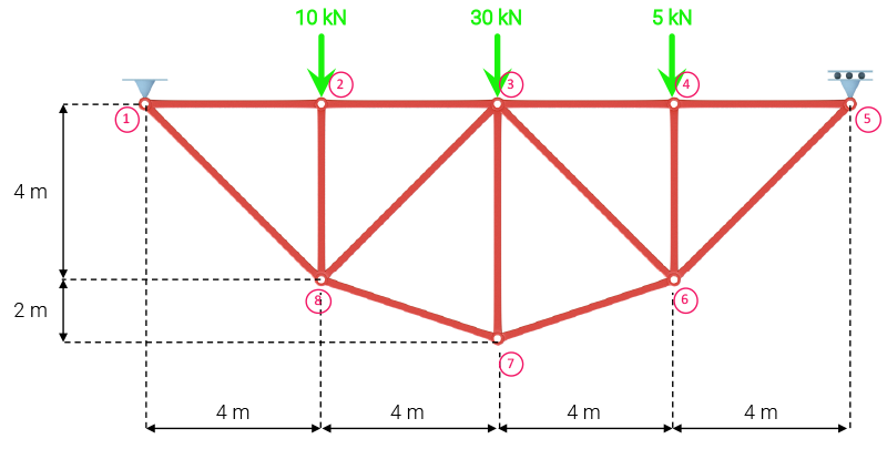
Fig 1. Inverted bowstring truss from lecture 53 of The Direct Stiffness Method for Truss Analysis with Python course.

If you’ve completed this course, then you know that in order to complete the analysis of this truss using the direct stiffness method, we went through the following steps:

• we started by defining the structures’ nodal coordinates, elements, restrained degrees of freedom and applied loading
• we calculated the orientation and length of each member
• we calculated the global stiffness matrix for each element
• we combined these element stiffness matrices into a primary stiffness matrix for the structure and subsequently refined this to a structure stiffness matrix by layering on knowledge of the restrained degrees of freedom.
• then, we inverted the stiffness matrix and multiplied it by the external force vector to obtain the displacement for each degree of freedom.
• from here, we did some post-processing to determine member forces and reactions.

This is the fundamental finite element analysis procedure that we’ve explored and expanded on across many courses. And while it’s important to understand how it works, there’s no harm in implementing pre-existing libraries once you do!

The output of this analysis can be summarised as follows; the nodal displacements Ux and Uy for each node are:

NODAL DISPLACEMENTS
Node 1: Ux = 0.0 m, Uy = 0.0 m
Node 2: Ux = -0.0001 m, Uy = -0.00063 m
Node 3: Ux = -0.00019 m, Uy = -0.00073 m
Node 4: Ux = -0.00028 m, Uy = -0.00057 m
Node 5: Ux = -0.00036 m, Uy = 0.0 m
Node 6: Ux = -5e-05 m, Uy = -0.00055 m
Node 7: Ux = -0.00018 m, Uy = -0.00058 m
Node 8: Ux = -0.00032 m, Uy = -0.00059 m

The axial forces in the truss elements are as follows, with negative numbers indicating compression.

MEMBER FORCES
Force in member 1 (nodes 1 to 2) is -23.75 kN
Force in member 2 (nodes 2 to 3) is -23.75 kN
Force in member 3 (nodes 3 to 4) is -21.25 kN
Force in member 4 (nodes 4 to 5) is -21.25 kN
Force in member 5 (nodes 5 to 6) is 30.05 kN
Force in member 6 (nodes 6 to 7) is 27.95 kN
Force in member 7 (nodes 7 to 8) is 27.95 kN
Force in member 8 (nodes 1 to 8) is 33.59 kN
Force in member 9 (nodes 2 to 8) is -10.0 kN
Force in member 10 (nodes 3 to 7) is -25.0 kN
Force in member 11 (nodes 4 to 6) is -5.0 kN
Force in member 12 (nodes 3 to 8) is -1.77 kN
Force in member 13 (nodes 3 to 6) is -5.3 kN

Our task now is to start with the same model definition data and, instead of implementing our own solution algorithm, arrive at the same result using OpenSeesPy.

3.1 Basic setup

In case you haven’t completed the truss analysis course mentioned already, here’s a quick recap of how we define our structure at the start of the code.

We start by simply defining the material Young’s modulus and cross-sectional area of the truss members as two constants. We’re assuming the same values for each member although it’s trivial to introduce different values for each truss member.

#Constants
E = 200*10**9 #(N/m^2)
A = 0.005 #(m^2)

Next we define the x and y coordinates of each node in a 2D Numpy array.

#Nodal coordinates [x, y]
nodes = np.array([[0,6],
                  [4,6],
                  [8,6],
                  [12,6],
                  [16,6],
                  [12,2],
                  [8,0],
                  [4,2]
                 ])

Probably the most important definition is the member definition or connectivity; again, we use a 2D Numpy array to store the id of the node at each end of each member. This is all much easier to interpret if you start with a clearly labelled diagram, see Fig 1 above.

#Members [node_i, node_j]
members = np.array([[1,2],
                   [2,3],
                   [3,4],
                   [4,5],
                   [5,6],
                   [6,7],
                   [7,8],
                   [1,8],
                   [2,8],
                   [3,7],
                   [4,6],
                   [3,8],
                   [3,6]
                   ])

It’s worth pointing out that the process of generating the data that goes into the nodes and members array was manual, for want of a better term. I started by sketching out the truss and working out the nodal coordinates on paper. This doesn’t scale well for larger structures so in our 3D Space Frame Analysis using Python and Blender course, we walk through how to use the free open-source 3D modelling tool, Blender, to generate model data. You could easily apply what we did in that course to speed up the process of generating geometry data for your models.

In our original direct stiffness method code, we also defined the restrained degrees of freedom (for supports) and we built the external force vector. Since we’re using OpenSeesPy, this will be a little more straightforward here.

3.2 Plotting the structure

It’s always a good idea to visualise the structure, once you’ve defined it. So, just like we did in our original code, we’ll plot the truss we’ve just defined, using matplotlib. We start by importing matplotlib at the top of our notebook (I’m doing all of this inside a Jupyter Notebook BTW). While we’re at it we can import numpy and math.

import math
import numpy as np
import matplotlib.pyplot as plt

The code to plot the structure is pretty simple; after initialising a figure and setting the axes to have equal scales, we cycle through each member and plot a blue line for each. The we do some housekeeping to tidy the plot up with a title, grid and axis labels.

fig = plt.figure()
axes = fig.add_axes([0.1,0.1,3,3])
fig.gca().set_aspect('equal', adjustable='box')

#Plot members
for mbr in members:
    node_i = mbr[0] #Node number for node i of this member
    node_j = mbr[1] #Node number for node j of this member

    ix = nodes[node_i-1,0] #x-coord of node i of this member
    iy = nodes[node_i-1,1] #y-coord of node i of this member
    jx = nodes[node_j-1,0] #x-coord of node j of this member
    jy = nodes[node_j-1,1] #y-coord of node j of this member

    axes.plot([ix,jx],[iy,jy],'b') #Member

#Plot nodes
for n in nodes:
    axes.plot([n[0]],[n[1]],'bo')

axes.set_xlabel('Distance (m)')
axes.set_ylabel('Distance (m)')
axes.set_title('Structure to analyse')
axes.grid()
plt.show()

The result is…

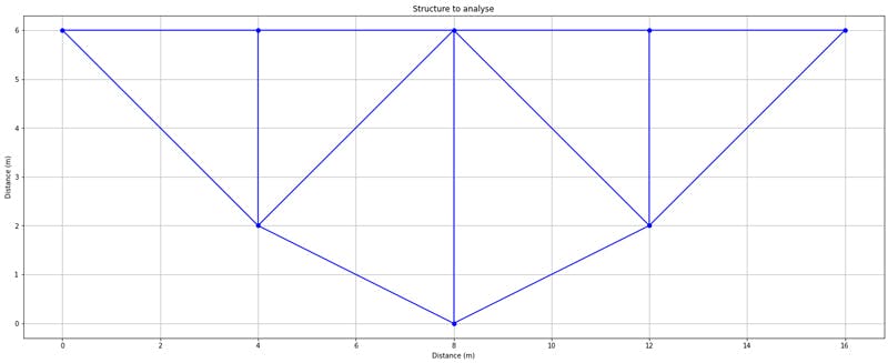
Fig 2. Initial undeformed structure.

3.3 Model definition in OpenSeesPy

Before we move on to use OpenSeesPy in our Jupyter Notebook, you’ll likely need to download it. You can refer to the docs here, but it’s just a matter of installing from the terminal (I’m on a Mac), like any other package…

pip install openseespy

Then import it at the top of your notebook (or .py file if you’re not using a Jupyter Notebook) with the rest of your imports.

from openseespy.opensees import *

Before defining a new model, it’s sensible to remove any model that might already be in memory (for example if you’ve already run your code). We do this by calling wipe(). Then we initialise a model builder by specifying the model type, basic in this case, the number of dimensions (2) and number of degrees of freedom at each node (2).

#Remove any existing model
wipe()

#Set the model builder - 2 dimensions and 2 degrees of freedom per node
model('basic', '-ndm', 2, '-ndf', 2)

By calling model() we are given access to the other OpenSeesPy specific commands needed to define our nodes and members. See the original docs here for (not much) more information.

Defining Nodes

Next, we can define the nodes of our model with the node command. Be careful not to use node as a variable name elsewhere in your code! We can implement a simple for loop to cycle through each node in a nodes array and call the node() method on each. We pass in the node id and x and y coordinates to the node() method.

for i, n in enumerate(nodes):
    node(i+1, float(n[0]), float(n[1]))

Defining Elements

To define elements, we first need to define a material - we’ll define a uniaxialMaterial with type Elastic, material id equal to 1 and Young’s modulus set the the variable E that we defined above. Again, to dig a little deeper into the different options available, check out the relevant section in the OpenSees docs here. Note that the number of types and material behaviours you can specify is vast - just take a look at the linked docs to get a sense of what’s possible!

uniaxialMaterial("Elastic", 1, E)

Now we can implement the element() method in a for loop that cycles through each member in the members array. For each element, we’re specifying:

• The element type (Truss)
• Element id
• Node number at node i
• Node number at node j
• Cross-sectional area (A, defined above)
• Material id (the id of the uniaxial material we just defined)

for i, mbr in enumerate(members):
    element("Truss", i+1, int(mbr[0]), int(mbr[1]), A, 1)

Again, for reference, here is the relevant section of the docs for the element command.

Defining boundary conditions

Defining the boundary or support conditions is very simple, we can call the fix() method and pass the node id and 1 or 0 to indicate fixity or not for the x and y degree of freedom. So, in our case to add a pin at node 1 and a horizontal roller at node 5 is as simple as…

# Set boundary condition
fix(1,1,1) #Pin at node 1
fix(5,0,1) #Horizontal roller at node 5

This completes the model definition - as you can see, provided we have a way to generate the data that defines the geometry of the structure, defining the model is very fast!

3.4 Load definition in OpenSeesPy

The process of applying loads to our model is a three step procedure. The fact that there are three steps is an indication of the degree of complexity that we can achieve when applying static and, in particular, dynamic loads in OpenSeesPy.

We start by defining a time series - in our case we’re applying constant magnitude static loads so we can simply define a constant time series with an id of 1. Further detail and details of alternative time series can be found here.

timeSeries("Constant", 1)

Next, we create a load pattern associated with our time series. Here we will define a Plain load pattern with a pattern tag of 1, and associated with the time series with id or tag equal to 1. More details here.

pattern("Plain", 1, 1)

Finally, we get to the more intuitive step which involves specifying loads and their locations - this is mercifully straightforward - we call load and pass the node location and the x and y force components. So, referring to our original problem definition in Fig. 1, we have…

load(2, 0.0, -10000.0)
load(3, 0.0, -30000.0)
load(4, 0.0, -5000.0)

3.5 OpenSeesPy Analysis

The analysis process consists of the following 7 commands, which allow us to tune the solution procedure. As we’re performing a relatively simple (linear static) analysis, we’ll be using a relatively straightforward configuration. But keep in mind that the following commands allow huge flexibility to tailor the analysis for quite complex analyses.

We first call system to construct the solver object that is used to store and solve the system of simultaneous equations - much like we did in our implementation of the direct stiffness method. We specify BandSPD which dictates how the equations in the solver will be constructed. More details in the OpenSees docs here and the OpenSeesPy docs here.

system("BandSPD")

Then we call the numberer command (docs) which essentially controls how degrees of freedom are numbered. We pass the argument RCM to indicate we will be using the Reverse Cuthill-McKee Numberer.

numberer("RCM")

We establish a constraint handler next in order to specify how the constraint equations are enforced in the analysis (Doc ref). We specify Plain which is suitable for the single point constraints we have on our structure.

constraints("Plain")

Then we define an integrator object - this is used to define how the model responds to the applied loads or displacements during an analysis. It determines how the solution to the governing equations is obtained at each step of the analysis.

We specify a LoadControl integrator as it’s one of the simplest and well-suited to static analyses. The 1.0 indicates that for each increment in the load application, the full load specified in the load pattern will be applied. In effect, we are defining the instantaneous application of the full load in one time step, a classic linear static analysis. Docs ref.

integrator("LoadControl", 1.0)

Next, we can specify the solution algorithm to use - we will specify Linear - one of the most basic and straightforward solution algorithms and again, well suited to our simple case study analysis. Docs ref.

algorithm("Linear")

Then we can specify the analysis type - Static in our case. Obviously we are ignoring any dynamic effects and assuming all loads are applied slowly such that inertia forces are negligible. Docs ref.

analysis("Static")

Finally, we can kick off an analysis based on the previously defined model, analysis type, integrator and solution algorithm. We can specify the number of analysis steps as an argument. Since we’re performing a linear static analysis, we can specify a single analysis step.

analyze(1)

After calling these configuration methods, assuming we haven't messed up any of our config steps, we whould have our solution and all that remains is to extract the results, perform any post-processing, visualise them...and, of course, confirm that they agree with our original analysis results!

3.6 OpenSeesPy Results

Now we’re finally in a position to extract some results from our OpenSeesPy analysis! We’ll extract nodal displacements and then the element forces. We’ll compare these with our original direct stiffness method analysis and finally implement a simple plot to visualise the deformed structure.

Nodal Displacements

We can extract the x and y components of displacement for each node using the nodeDisp command and specifying the node number and whether we want the horizontal or vertical component. We’ll call this in a loop iterating over each node in the nodes array. We’ll also print out the displacements to compare with our earlier analysis.

for i, n in enumerate(nodes):
    ux = round(nodeDisp(i+1, 1),5) #Horizontal nodal displacement
    uy = round(nodeDisp(i+1, 2),5) #Vertical nodal displacement
    print(f'Node {i+1}: Ux = {ux} m, Uy = {uy}')

This results in the following output:

Node 1: Ux = 0.0 m, Uy = 0.0
Node 2: Ux = -0.0001 m, Uy = -0.00063
Node 3: Ux = -0.00019 m, Uy = -0.00073
Node 4: Ux = -0.00028 m, Uy = -0.00057
Node 5: Ux = -0.00036 m, Uy = 0.0
Node 6: Ux = -5e-05 m, Uy = -0.00055
Node 7: Ux = -0.00018 m, Uy = -0.00058
Node 8: Ux = -0.00032 m, Uy = -0.00059

Now, if we compare with our earlier analysis output, we can see that the nodal displacements agree perfectly - so we’ve essentially completed our mission! We’ve implemented a simple 2D linear static truss analysis using OpenSeesPy.

Plotting the deflected shape

We can re-use some code from our earlier analysis to plot the deflected shape of the structure. This is achieved in much the same way as our earlier plot except this time we also plot the members after they’ve been moved according to the nodal displacement from our analysis. Note that we amplify our displacements by a factor, xFac=500 so that they’re visible in our plot.

fig = plt.figure()
axes = fig.add_axes([0.1,0.1,2,2])
fig.gca().set_aspect('equal', adjustable='box')

xFac=500

#Plot members
for mbr in members:
    node_i = int(mbr[0]) #Node number for node i of this member
    node_j = int(mbr[1]) #Node number for node j of this member

    ix = nodes[node_i-1,0] #x-coord of node i of this member
    iy = nodes[node_i-1,1] #y-coord of node i of this member
    jx = nodes[node_j-1,0] #x-coord of node j of this member
    jy = nodes[node_j-1,1] #y-coord of node j of this member

    axes.plot([ix,jx],[iy,jy],'grey', lw=0.75) #Member

    ux_i = nodeDisp(node_i, 1) #Horizontal nodal displacement
    uy_i = nodeDisp(node_i, 2) #Vertical nodal displacement
    ux_j = nodeDisp(node_j, 1) #Horizontal nodal displacement
    uy_j = nodeDisp(node_j, 2) #Vertical nodal displacement

    axes.plot([ix + ux_i*xFac, jx + ux_j*xFac], [iy + uy_i*xFac, jy + uy_j*xFac],'r') #Deformed member

axes.set_xlabel('Distance (m)')
axes.set_ylabel('Distance (m)')
axes.set_title('Deflected shape')
axes.grid()
plt.show()

This yields the following (amplified) deflected shape shown in red with the original structure shown in grey.

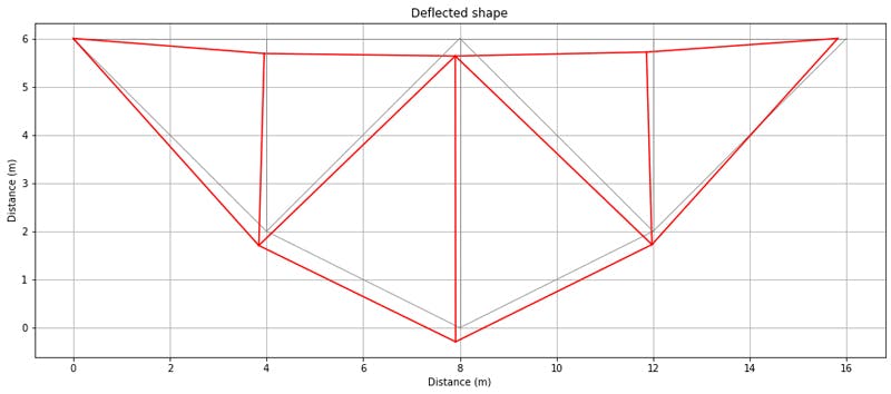
Fig 3. Deflected shape.

Axial forces

For completeness, we’ll also extract the member axial forces and compare them with our earlier model.

The relevant OpenSees command for extracting the axial force in each member is basicForce, so for example,

basicForce(5) #Element force in member 5 (nodes 5-6)

would output,

[30052.038200428327]

We can now call this function in a for loop for each member, saving the force value for use later. Note that the basicForce command returns a list with the axial force in the member as the first (and only) element. So we need to extract this element and round it to 2 decimal places.

mbrForces = np.array([])
for i, mbr in enumerate(members):
    axialForce = round(basicForce(i+1)[0]/1000,2)
    mbrForces = np.append(mbrForces,axialForce) #Store axial loads
    print(f'Force in member {i+1} (nodes {mbr[0]} to {mbr[1]}) is {axialForce} kN')

So the output from this post-processing step is…

Force in member 1 (nodes 1 to 2) is -23.75 kN
Force in member 2 (nodes 2 to 3) is -23.75 kN
Force in member 3 (nodes 3 to 4) is -21.25 kN
Force in member 4 (nodes 4 to 5) is -21.25 kN
Force in member 5 (nodes 5 to 6) is 30.05 kN
Force in member 6 (nodes 6 to 7) is 27.95 kN
Force in member 7 (nodes 7 to 8) is 27.95 kN
Force in member 8 (nodes 1 to 8) is 33.59 kN
Force in member 9 (nodes 2 to 8) is -10.0 kN
Force in member 10 (nodes 3 to 7) is -25.0 kN
Force in member 11 (nodes 4 to 6) is -5.0 kN
Force in member 12 (nodes 3 to 8) is -1.77 kN
Force in member 13 (nodes 3 to 6) is -5.3 kN

…which agrees perfectly with our original analysis - no surprise there considering the nodal displacements have already been shown to agree.

Plotting tension/compression member

As the very final step, we can plot the structure again with the members colour-coded - red for compression and blue for tension.

fig = plt.figure()
axes = fig.add_axes([0.1,0.1,2,2])
fig.gca().set_aspect('equal', adjustable='box')

#Plot members
for n, mbr in enumerate(members):
    node_i = mbr[0] #Node number for node i of this member
    node_j = mbr[1] #Node number for node j of this member

    ix = nodes[node_i-1,0] #x-coord of node i of this member
    iy = nodes[node_i-1,1] #y-coord of node i of this member
    jx = nodes[node_j-1,0] #x-coord of node j of this member
    jy = nodes[node_j-1,1] #y-coord of node j of this member

    if(abs(mbrForces[n])<0.001):
        axes.plot([ix,jx],[iy,jy],'grey',linestyle='--') #Zero force in member
    elif(mbrForces[n]>0):
        axes.plot([ix,jx],[iy,jy],'b') #Member in tension
    else:
        axes.plot([ix,jx],[iy,jy],'r') #Member in compression

axes.set_xlabel('Distance (m)')
axes.set_ylabel('Distance (m)')
axes.set_title('Tension/compression members')
axes.grid()
plt.show()

This yields the following plot…

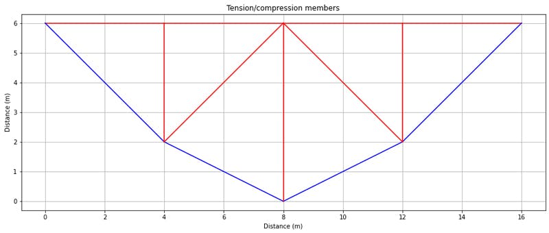
Fig 4. Tension (blue) and compression (red) members.

4.0 Conclusion

This wraps up our case study analysis! To summarise, we’ve performed a linear static 2D truss analysis using OpenSeesPy and confirmed agreement with our original stiffness method analysis from the The Direct Stiffness Method for Truss Analysis with Python course.

As I said at the outset, we’ve barely scratched the surface of what can be achieved with OpenSeesPy. My hope is that after working through this tutorial, you’re motivated to dive a little deeper into OpenSeesPy to explore what else you can achieve! If you're hungry for more OpenSeesPy content, check out this tutorial where we analyse a 2D portal frame structure...a great next step after you've completed this tutorial.

I look forward to doing the same and reporting back with more tutorial articles like this one.

If you’re not yet ready to dive into using ‘black box’ analysis tools and what to get a better understanding of how to implement these matrix-based analysis methods, from first principles, then the place to start is the truss analysis course I’ve referenced throughout this tutorial. If you want to achieve the same thing, but for 3D trusses or spaceframes, then take a look at 3D Space Frame Analysis using Python and Blender. In this course we also explore model data generation in Blender - which is a game changer once you get beyond small toy models.

Ok, that’s all for now and indeed that's all for 2023 - see you in the next one in 2024 🎉!