OpenSeesPy Quick Start - Build a Parametric Continuous Beam Calculator (with hinges)

1.0 Introduction

In this tutorial, we’ll build a continuous beam analysis script using OpenSeesPy. We'll also build in the ability to specify rotational hinges within our continuous beam.

Multi-span continuous beams are so common that it makes sense to have a script in our toolbox to very quickly generate the shear force diagram, bending moment diagram, reactions and deflected shape.

Analysing them by hand takes forever, and even setting them up for analysis in commercial software packages can feel needlessly laborious. This is where having a simple analysis script comes in handy - quickly plug in the beam geometry and loading information, hit Run, and you’re done!

Once you complete this tutorial, you’ll have built this script. Work through it with me now, step by step, or download the completed code from the resource panel above.

If you prefer a video run-through to reading, I have a full tutorial video that walks through each code block 👇

This is one of a number of tutorials on EngineeringSkills exploring the OpenSeesPy library. If you’re completely new to OpenSeesPy, go back to the first tutorial here, where I introduce the library.

This continuous beam project follows on very closely from this tutorial where we analysed a simple 2D moment frame. Make sure to check that out before you work through this. In fact, the OpenSeesPy portion of the build will be very similar - what’s new in this tutorial is:

1. how we handle some of the structure parameterisation,
2. the inclusion of rotation hinges.

Our plan will be to define the structural parameters (material, geometry and loading) first. Then we’ll dive into building the OpenSeesPy model, tackling the parameterisation as we define various parts of the model.

Ok, let’s get into the build!

2.0 Parameterising the Continuous Beam

Versions:
openseespy: openseespy 3.7.1.2
opsvis: opsvis 1.3.4
numpy: numpy 1.26.4
matplotlib: matplotlib 3.9.4

import openseespy.opensees as ops
import opsvis as opsv
import numpy as np
import matplotlib.pyplot as plt

Our goal is to have the entire definition of the structure parameterised. All this really means is that we want to be able to define everything at the start of the script and then let the code handle the OpenSeesPy model building process.

We can start by defining the material and geometric properties of the cross-section:

• Young’s Modulus for the beam material (we’ll assume steel), $E$
• Cross-sectional area of the continuous beam section, $A$
• Second moment of area about the major principle axis of the section, $I_z$

#Constants
E = 200*10**9   #(N/m^2) Young's Modulus
A = 0.03        #(m^2) Cross-sectional area
Iz = 300*10**-6 #(m^4) Second moment of area

We’ll define the overall span of the beam next. Note that this is the entire beam length and ignores the positions of supports. We’ll start by assuming a $10\:m$ beam.

L = 10 #(m) Total beam length

Next we define the positions of supports as well as the degree of restraint provided by each. The data for one support will be stored in a list consisting of 4 numbers:

• The first number indicates the location of the support
• The second indicates the whether or not the support provides horizontal translational restraint
• The third indicates the whether or not the support provides vertical translational restraint
• The fourth indicates the whether or not the support provides rotational restraint.

Restraint is indicated by the number 1 with no restraint indicated by 0. So for example, [1, 1, 1, 0] defines a pin support located $1\:m$ along the beam, assuming the origin is at the left-most tip of the beam.

We can store the support data in a 2D numpy array called r. So, in our case we define 4 supports as follows:

#Restraints [pos, Ux_Restraint, Uy_Restraint ThetaZ_Restraint]
r = np.array([
	[1, 1, 1, 0], #Pin
	[4, 0, 1, 0], #Roller
	[7, 0, 1, 0], #Roller
	[9, 0, 1, 0], #Roller
])

We take a similar approach when defining the loading information. Each action on the structure is defined by an array of numbers with all actions applied to the structure being collected into a single array. We define point actions (point moments and forces) first. The first number in an individual action record indicates the location of the action. The remaining numbers are the magnitude of the force in each orthogonal direction (x, then y) and the moment magnitude.

#Point Forces and Moments [pos, Fx, Fy, Mz]
p = np.array([
	[3, 0., -30000., 0.],
	[5, 0., -10000., 0.],
	[5, 0., 0., 5000.]
])

Distributed loads are similarly defined. Note that we can define both uniformly distributed loads (UDLs) and loads of linearly varying intensity (a.k.a. trapezoidal loads), by specifying a different beginning and ending intensity. The first number in an individual load record indicates the start position of the load. The second number indicates the end position of the load. The third and fourth numbers indicate the start and end intensity of the load respectively. In our case, we define one UDL and one trapezoidal load that span the entire length of the beam.

#Distributed Forces [pos_start, pos_end, intensity_start, intensity_end]
w = np.array([
	[0, 10, -20000, -20000], #UDL
	[0, 10, 0, -5000] #Linear Load
])

Next, we can specify the location of additional nodes we want in the structure. These are particularly helpful as query locations, i.e. we can place a node at any specific location where we want to know the values of shear, moment and deflection. For example, here we place a query node at $0.5\:m$, $2\:m$ and $6.25\:m$ along the beam.

#Add nodes at specific query locations
q = np.array([0.5, 2, 6.25])

Finally, we can specify the location of any rotational hinges we want to place in the beam. These hinges act as rotational releases within the structure, effectively reducing the degree of determinacy by 1. If you’ve spent any time building shear and moment diagrams manually with hand calculations, you should be very familiar with this concept. Here, we place a hinge at $7.5\:m$ along the beam.

# Rotational hinge location
h = np.array([7.5])

With our structure and loading fully defined, we can move onto building our OpenSeesPy model.

3.0 Initialising the Model and Defining the Structure

As we’ve already seen in previous tutorials, the OpenSeesPy part of our script always starts the same way, we wipe any pre-existing model from memory and then define the model parameters; notably the number of dimensions (2 in our case) and number of degrees of freedom per node (3).

ops.wipe()
ops.model('basic', '-ndm', 2, '-ndf', 3)

3.1 Node locations list

Defining our nodes is probably the first time in this build where we actually have to start thinking about parameterisation. We will define a node at the location of:

• the start and end of the beam
• each restraint
• each point action (force or moment)
• the start and end position of each distributed load
• each query location
• each hinge location

With this approach, we can easily define beam elements between each node at a later stage. We start by defining an array, nodeLocations to store the location of each node. Then, we can cycle through the various arrays defined previously, appending node positions as required. The last step in building our list of node locations is to remove any duplicate locations and sort the list.

# Initialse the array with entries for start and end of beam
nodeLocations = np.array([0, L])

# Add nodes at each restraint location
nodeLocations = np.append(nodeLocations, r[:, 0])

# Add nodes at each point action location
if len(p)>0: nodeLocations = np.append(nodeLocations, p[:, 0])

# Add node at start and end of each distributed load
if len(w)>0: nodeLocations = np.append(nodeLocations, np.concatenate((w[:, 0], w[:, 1])))

# Add node at each query location
if len(q)>0: nodeLocations = np.append(nodeLocations, q)

# Add node at each rotational hinge location
if len(h)>0: nodeLocations = np.append(nodeLocations, h)

# De-duplicate and sort
nodeLocations = np.unique(nodeLocations)
nodeLocations.sort()

3.2 Defining the nodes

The inclusion of hinges within our model slightly complicates how we define our nodes. To see why, we first need to discuss how rotational hinges are implemented.

The first thing we do is define a set containing the locations of each of our hinges (if we have any). This will allow us to quickly test whether a node at a given location should be a hinge or not.

hingeLocations = set(float(x) for x in h) if len(h) > 0 else set()

Next, we want to define a dictionary that maps each node’s location to the OpenSeesPy nodeTag for that node. Since we may have two nodes at the same location (if that location has a hinge), we need two versions of our mapping.

Both will map locations to nodeTags, but in the case that we have a hinge at a location, one mapping (loc2tagL) will record the ‘left’ nodeTag at the hinge location. The other mapping (loc2tagR) will record the ‘right’ nodeTag at the hinge location.

Before iterating through our list of node locations, we define the empty dictionaries:

# Maps from location -> node tag(s)
loc2tagL = {}
loc2tagR = {}

Then we can initialise an integer to keep track of the nodeTags as each new node is defined. In our main loop, we can check if the current location is a hinge location (member of our hingeLocations set). If it is, we define two nodes at the location.

If not, we simply define one node. Each time we define a new node in OpenSeesPy, we use the ops.node() command and pass in the nodeTag, and x and y coordinates of the node. The complete node-defining loop is as follows:

# Create nodes (duplicate at hinges)
nodeTag = 0
for i, n in enumerate(nodeLocations):
	xCoord = float(n)

	if xCoord in hingeLocations:
		# Left node at hinge
		nodeTag += 1
		tagL = int(nodeTag)
		ops.node(tagL, xCoord, 0.0)

		# Right node at hinge (coincident)
		nodeTag += 1
		tagR = int(nodeTag)
		ops.node(tagR, xCoord, 0.0)

		#Update mapping
		loc2tagL[xCoord] = tagL
		loc2tagR[xCoord] = tagR
	else:
		nodeTag += 1
		tag = int(nodeTag)
		ops.node(tag, xCoord, 0.0)

		#Update mapping
		loc2tagL[xCoord] = tag
		loc2tagR[xCoord] = tag

Printing the mappings helps clarify how they work:

print(loc2tagL)
print(loc2tagR)

This gives us:

{0.0: 1, 0.5: 2, 1.0: 3, 2.0: 4, 3.0: 5, 4.0: 6, 5.0: 7, 6.25: 8, 7.0: 9, 7.5: 10, 9.0: 12, 10.0: 13}

{0.0: 1, 0.5: 2, 1.0: 3, 2.0: 4, 3.0: 5, 4.0: 6, 5.0: 7, 6.25: 8, 7.0: 9, 7.5: 11, 9.0: 12, 10.0: 13}

Note that both dictionaries are the same except for the key 7.5, where loc2TagL maps to a nodeTag value of 10 and loc2TagR maps to node tag 11.

3.3 Applying the hinge constraint

Now that our OpenSeesPy command contains all of the required nodes, we can apply the hinge constraint between nodes 10 and 11 at the hinge location (x=7.5). This is achieved with the ops.equalDOF() command.

We want to tie the two translational degrees of freedom, so we pass in the relevant node numbers and the arguments 1 and 2, referencing the first two degrees of freedom.

# Apply hinge constraints: tie translations only (Ux=1, Uy=2), release rotation (Rz=3)
for xCoord in hingeLocations:
	ops.equalDOF(loc2tagL[xCoord], loc2tagR[xCoord], 1, 2)

3.4 Defining beam elements

As we saw previously, we need to start the element definition process by first defining a linear geometric transform. You can refer to the previous tutorial for more details on what this is, but basically, we are defining a linear transformation between the beam element’s local reference frame and the global reference frame. This becomes more significant for controlling the orientation of elements on larger 3D models - for our continuous beam model, it’s a trivial, but necessary step.

transfType = 'Linear'
transfTag = 1
ops.geomTransf(transfType, transfTag)

Now we can define a beam element between each successive pair of nodes. One thing to note is that any beam element immediately to the left of a hinge must have its right-hand end defined using the nodeTag defined in the left-side mapping for that location. Similarly, the beam element immediately to the right of a hinge, must have its left-hand end defined using the nodeTag recorded in the right-side mapping.

For us, this means the element to the left of the hinge is defined by nodeTags 9 and 10, while the adjoining element to the right of the hinge is defined by nodeTags 11 and 12. The individual beam elements are defined using the ops.element() command that we saw in the previous tutorial.

# Define beam elements
for n in range(len(nodeLocations)-1):
	startPos = nodeLocations[n]
	endPos   = nodeLocations[n+1]

	# Key rule:
	# - element starts on the "right" tag of the start position
	# - element ends on the "left" tag of the end position
	startNode = loc2tagR[startPos]
	endNode   = loc2tagL[endPos]

	eleTag = n+1

	ops.element('elasticBeamColumn', eleTag, startNode, endNode, A, E, Iz, transfTag)

3.5 Defining restraints

Restraints are defined by cycling through the restraints array, and for each restraint, we use its location to identify the relevant nodeTag, we can build a tuple representing the restraint for each degree of freedom and pass this information into the ops.restraint() command.

for i, R in enumerate(r):
	location = R[0] #Restraint location
	nodeTag = loc2tagL[location]  # use left tag by default

	nodeFixity = (nodeTag, *(int(x) for x in R[1:]))
	ops.fix(*nodeFixity) #Define restraint using fixity specified

Although not completely necessary, we’ll follow the same practice as in the last tutorial and use OpsVis to visually confirm our model at each stage. We can easily define a function that uses OpsVis to plot the structure. We then immediately call our function.

# Print model to confirm visually
def plotStructure():
	opsv.plot_model(fig_wi_he=(50,20))
	plt.title('Beam')
	plt.xlabel('Distance (m)')
	plt.xticks(np.arange(0,L+1,1))
	ax = plt.gca()
	ax.tick_params(axis='y', labelleft=False)
	plt.grid()
	plt.show()

plotStructure()

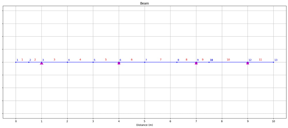
Fig 1. Structure (nodes, elements and restraints) visualised using OpsVis.

This allows us to confirm that the model we're building up in OpenSeesPy is consistent with the structure we defined in the previous section.

4.0 Defining Loads/Actions

Our loads are defined in a very similar way to nodes and elements, generally we can just cycle through the user-defined loading data and define the loads as needed. The process of defining linearly varying loads is slightly more involved - but still pretty straightforward.

Before we define individual actions on the structure, we start in the usual way by defining a timeseries and pattern.

# Create TimeSeries with a tag of 1
ops.timeSeries("Constant", 1)

# Create a plain load pattern associated with the TimeSeries
# (pattern, patternTag, timeseriesTag)
ops.pattern("Plain", 1, 1)

4.1 Point forces/moments

Let’s start with an easy one - point actions. We cycle through each point action defined by the user and using the same patterns we’ve seen above, we define each load.

for P in p:
	location = P[0] #Action location
	nodeTag = int(loc2tagL[location])  #apply to left tag by default

	loadDefinition = (nodeTag, *P[1::])
	ops.load(*loadDefinition)

This only leaves distributed loads to deal with. We'll break this into a two separate operations:

• One for uniformly distributed loads (easier)
• And one for linearly varying distributed loads (slightly more involved)

4.2 Uniformly distributed loads (UDLs)

We cycle through each distributed load definition and after checking the start and end magnitude to make sure they’re the same, we extract the start and end positions. This allows us to identify the index of the node located at the start and end position of the current uniformly distributed load.

Our next task is to determine which beam elements lie between these start and end nodes as these, and only these beam elements will have the current UDL applied to them. To do this, we cycle through the nodeLocations array as a means of iterating over each element and extracting the elementTag. While looping through nodeLocations, we check

• if the startNode for the current element is greater than or equal to startNodeLoad (the start node for the current load), AND
• if the endNode for the current element is less than or equal to endNodeLoad (the end node for the current element).

If both conditions are met, then we know that the current beam element lies within the boundaries of the current UDL and therefore we need to apply this UDL to the beam element.

for W in w:
	# Only process uniformly distributed loads in this block
	if W[2] == W[3]:
		startLocation = W[0]
		endLocation   = W[1]

		# Find location indices in nodeLocations
		startIndexLoad = np.where(nodeLocations == startLocation)[0].item()
		endIndexLoad = np.where(nodeLocations == endLocation)[0].item()

		# Apply load to each element fully within the extents
		# Element with tag (n+1) spans nodeLocations[n] -> nodeLocations[n+1]
		for n in range(startIndexLoad, endIndexLoad):
			eleTag = int(n+1)
			ops.eleLoad('-ele', eleTag, '-type', '-beamUniform', float(W[2]))

4.3 Linearly varying distributed loads (LVDLs)

With UDLs under our belt, it will be easier to understand how to apply linearly varying distributed loads (LVDLs). We again start by cycling through each distributed load but this time we filter to identify only loads where the start magnitude doesn't match the end magnitude.

We identify the node index at the start and end of the LVDL as above. This time we also determine the slope or rate of change of the load intensity. We cycle through each beam element as we did before, checking if the element lies within the boundaries of the LVDL.

The extra step this time is that each time we apply the LVDL to a beam element, we need to identify the magnitude at the start and end of the beam element. For this we use information on the start/end position of the element, the starting magnitude of the LVDL, defined by the user and the rate of change of the LVDL, calculated above.

With this information we can apply the LVDL using the eleLoad command used for UDLs. Now, if you look in the OpenSeesPy docs for eleLoad, you won't find any information about how to apply a LVDL! It turns out that this is an undocumented (currently) feature of this method.

Rather than me repeating the explanation of this undocumented feature of the method here, you can read my source here which lays it out very clearly. To apply the LVDL using eleLoad, our function signature is as follows:

eleLoad('-ele', eleTag,'-type','beamUniform', wya,wxa,aOverL,bOverL,wyb,wxb)

where, in our case:

• wya is the magnitude of the LVDL that applies along an axis perpendicular to the beam element at the start of the beam element (the starting magnitude we defined at the top of the script)
• wxa is the magitude of the LVDL that applies along an axis parallel to the axis on the beam element (zero in our case)
• aOverL is the distance from the left side of the beam element to the start of the LVDL as a fraction of the total length of the element.
• bOverL, wyb and wxb all have meanings analogous to those above, but for the far side of the LVDL.

So, our complete code block for applying LVDLs is as follows:

for W in w:
	# Only process non-uniformly distributed loads in this block
	if W[2] != W[3]:
		startLocation = W[0]
		endLocation   = W[1]

		slope = (W[3]-W[2])/(W[1]-W[0])

		# Find location indices in nodeLocations (position-based, not nodeTag-based)
		startIndexLoad = np.where(nodeLocations == startLocation)[0].item()
		endIndexLoad   = np.where(nodeLocations == endLocation)[0].item()

		# Apply load to each element fully within the extents
		# Element with tag (n+1) spans nodeLocations[n] -> nodeLocations[n+1]
		for n in range(startIndexLoad, endIndexLoad):
			eleTag = int(n+1)

			# What is the position of start and end for this beam element
			startPosition = nodeLocations[n]
			endPosition   = nodeLocations[n+1]

			# Determine load magnitude at start of beam element
			startMag = W[2] + (slope * (startPosition - startLocation))

			# Determine load magnitude at end of beam element
			endMag   = W[2] + (slope * (endPosition - startLocation))

			# Apply linearly varying load to beam element
			ops.eleLoad('-ele', eleTag, '-type', 'beamUniform', float(startMag), 0, 0, 1, float(endMag), 0)

5.0 Analysis and Results

5.1 Analysis

Our analysis flow is exactly the same as for our previous tutorial example.

# Create SOE
ops.system('BandGeneral') # BandGeneral more general solver than 'BandSPD'

# Create DOF number
ops.numberer('RCM')

# Create constraint handler
ops.constraints('Transformation')

# Create integrator
ops.integrator('LoadControl', 1)

# Create algorithm
ops.algorithm('Linear')

# Create analysis object
ops.analysis('Static')

# Perform the analysis (with 1 analysis step)
ops.analyze(1)

And with that, our analysis is complete! All that remains is to visualise our results using OpsVis.

5.2 Results

We can start by defining functions that use OpsVis to plot the deflected shape, bending moment diagram and shear force diagram. For the shear force and bending moment diagrams, we'll pass in a scale factor to control the vertical scale of the plots.

Deflected shape function

def plotDEF():
	s = opsv.plot_defo(
		fig_wi_he=(50,20),
		fmt_defo={'color': 'red', 'linestyle': (0, (4, 5)), 'linewidth': 1.5},
		fmt_undefo={'color': 'green', 'linestyle': 'solid', 'linewidth': 2,},
	)
	plt.title('Deflection')
	plt.xlabel('Distance (m)')
	plt.xticks(np.arange(0,L+1,1))
	ax = plt.gca()
	ax.tick_params(axis='y', labelleft=False)
	plt.grid()
	plt.show()

Bending moment diagram function

def plotBMD(sFac):
	opsv.section_force_diagram_2d(
		'M', sFac, fig_wi_he=(50,20),
		fmt_secforce1={'color': 'green'},
		fmt_secforce2={'color': 'green'}
	)
	plt.title('Bending Moment Diagram')
	plt.xlabel('Distance (m)')
	plt.xticks(np.arange(0,L+1,1))
	ax = plt.gca()
	ax.tick_params(axis='y', labelleft=False)
	plt.grid()
	plt.show()

Shear force diagram function

def plotSFD(sFac):
	opsv.section_force_diagram_2d(
		'V', sFac, fig_wi_he=(50,20),
		fmt_secforce1={'color': 'red'},
		fmt_secforce2={'color': 'red'}
	)
	plt.title('Shear Force Diagram')
	plt.xlabel('Distance (m)')
	plt.xticks(np.arange(0,L+1,1))
	ax = plt.gca()
	ax.tick_params(axis='y', labelleft=False)
	plt.grid()
	plt.show()

Calling these functions and specifying custom scales...

plotDEF()
plotSFD(3.e-5)
plotBMD(5.e-5)

...yields the following results.

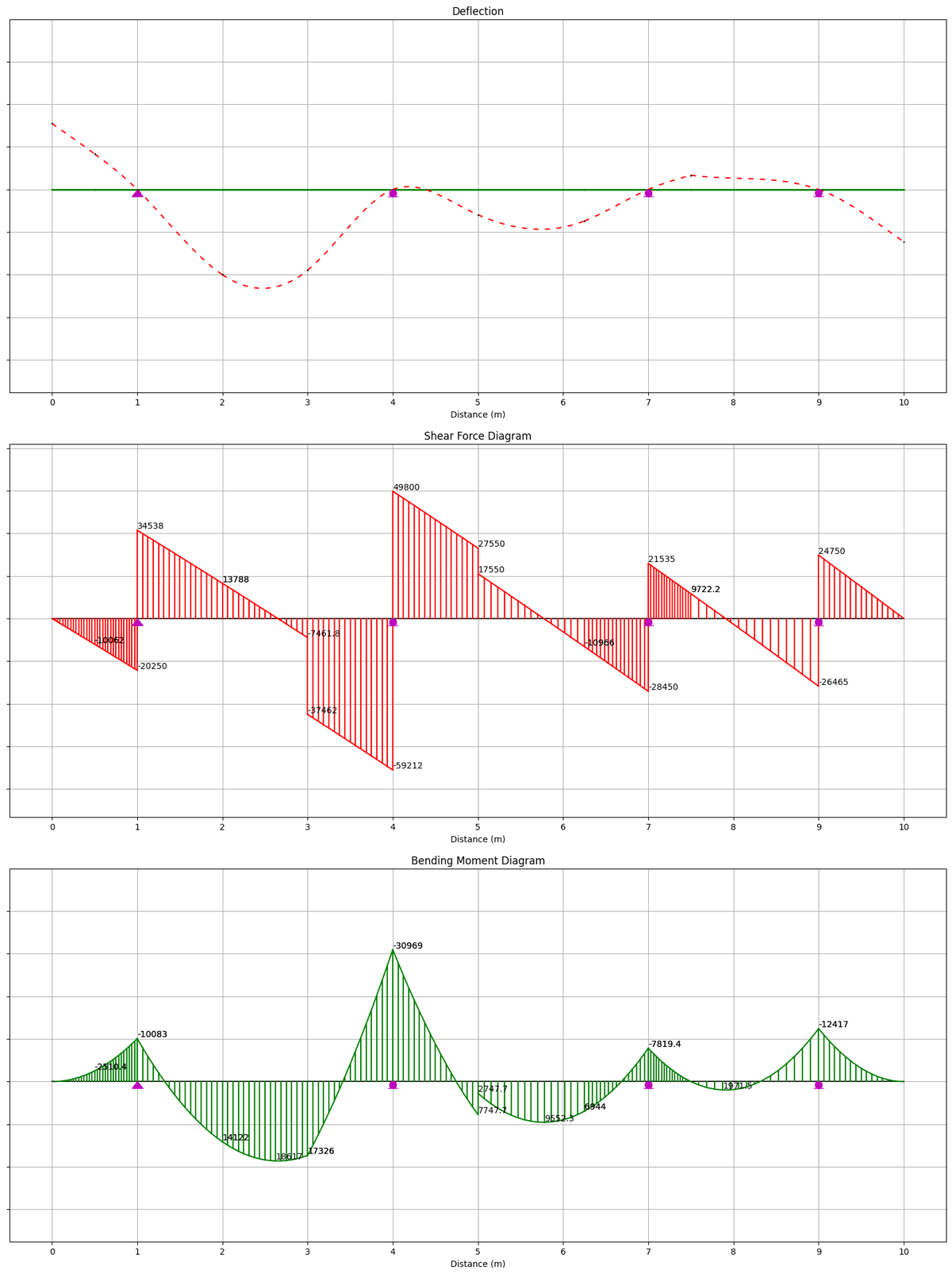
Fig 2. Deflected shape (top), annotated shear force diagram (middle), annotated bending moment diagram (bottom).

Reactions

Next, we'd like to extract the support reactions from the model. To do this we first need to calculate them by executing the OpenSeesPy command, reactions(). Then, we can access the reactions for a given nodeTag using the nodeReaction() command.

To obtain the reactions for each node, we can loop through the user-defined list specifying the reactions, identify the nodeTag that corresponds to each reaction location and then simply extract the reactions that correspond to that nodeTag. Finally, we summarise the reactions for each restraint by constructing and printing a string.

ops.reactions() #Calculate reactions

print("REACTIONS")
print('----------')

for i, R in enumerate(r):
	location = R[0] #Restraint location
	nodeTag = loc2tagL[location] # Left node by default (node that any restraint at this location was applied to)

	dofR = ops.nodeReaction(nodeTag) #Reactions for this node
	Rx = round(dofR[0]/1000,2)
	Ry = round(dofR[1]/1000,2)
	Mz = round(dofR[2]/1e6,2)
	print(f'Reactions at node {nodeTag}: Rx = {Rx} kN, Ry = {Ry} kN, Mz = {Mz} kNm')

This results in the following output:

REACTIONS
----------
Reactions at node 3: Rx = 0.0 kN, Ry = 54.79 kN, Mz = -0.0 kNm
Reactions at node 6: Rx = 0.0 kN, Ry = 109.01 kN, Mz = 0.0 kNm
Reactions at node 9: Rx = 0.0 kN, Ry = 49.98 kN, Mz = -0.0 kNm
Reactions at node 12: Rx = 0.0 kN, Ry = 51.22 kN, Mz = -0.0 kNm

We can also plot the reactions using OpsVis.

def plotReactions():
	opsv.plot_reactions(fig_wi_he=(50,20))
	plt.title('Reactions')
	plt.xlabel('Distance (m)')
	plt.xticks(np.arange(0,L+1,1))
	ax = plt.gca()
	ax.tick_params(axis='y', labelleft=False)
	plt.grid()
	plt.show()

plotReactions()

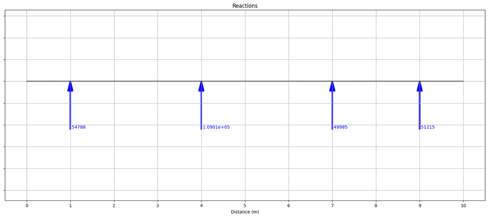
Fig 3. Reactions visualised using OpsVis.

Nodal displacements and rotations

As a final step, we’ll extract the nodal displacements and rotations - these are the only remaining quantitative results outstanding. This is achieved by again looping through nodeLocations and using the OpenSeesPy method nodeDisp to obtain the translations (Ux and Uy) and rotation (thetaZ) for each node. With the data extracted from the model, we can again construct a string to summarise the data for each node.

print('DISPLACEMENTS/ROTATIONS')
print("------------------------")
for i, x in enumerate(nodeLocations):
	tagL = loc2tagL[x]
	tagR = loc2tagR[x]

	# Always report left node
	delta = ops.nodeDisp(tagL)
	Ux = round(delta[0],10)
	Uy = round(delta[1],10)
	thetaZ = round(delta[2],6)

	print(f'Node {tagL} at {x} m: Ux = {Ux} m, Uy = {Uy} m, thetaZ = {thetaZ} rads')

	# If hinge (different tag), also report right node (rotations differ)
	if tagR != tagL:
		delta = ops.nodeDisp(tagR)
		Ux = round(delta[0], 10)
		Uy = round(delta[1], 10)
		thetaZ = round(delta[2], 6)
		print(f'Node {tagR} at {x} m: Ux = {Ux} m, Uy = {Uy} m, thetaZ = {thetaZ} rads')

This will result in the following output:

DISPLACEMENTS/ROTATIONS
------------------------
Node 1 at 0.0 m: Ux = 0.0 m, Uy = 0.0001516493 m, thetaZ = -0.000138 rads
Node 2 at 0.5 m: Ux = 0.0 m, Uy = 8.19336e-05 m, thetaZ = -0.000145 rads
Node 3 at 1.0 m: Ux = 0.0 m, Uy = 0.0 m, thetaZ = -0.000194 rads
Node 4 at 2.0 m: Ux = 0.0 m, Uy = -0.0001959877 m, thetaZ = -0.000131 rads
Node 5 at 3.0 m: Ux = 0.0 m, Uy = -0.0001857832 m, thetaZ = 0.00016 rads
Node 6 at 4.0 m: Ux = 0.0 m, Uy = 0.0 m, thetaZ = 7.7e-05 rads
Node 7 at 5.0 m: Ux = 0.0 m, Uy = -5.81083e-05 m, thetaZ = -8.6e-05 rads
Node 8 at 6.25 m: Ux = 0.0 m, Uy = -7.25101e-05 m, thetaZ = 7.7e-05 rads
Node 9 at 7.0 m: Ux = 0.0 m, Uy = 0.0 m, thetaZ = 8.5e-05 rads
Node 10 at 7.5 m: Ux = 0.0 m, Uy = 3.28643e-05 m, thetaZ = 5.7e-05 rads
Node 11 at 7.5 m: Ux = 0.0 m, Uy = 3.28643e-05 m, thetaZ = -2.7e-05 rads
Node 12 at 9.0 m: Ux = 0.0 m, Uy = 0.0 m, thetaZ = -6.9e-05 rads
Node 13 at 10.0 m: Ux = 0.0 m, Uy = -0.0001205858 m, thetaZ = -0.000138 rads

Remember, we have two nodes at the hinge location (7.5 m) - nodes 10 and 11. As expected, the vertical (and horizontal) translation is the same for both nodes, but the rotation is different which is the expected behaviour for a hinge.

At this point, we’ve completed our analysis. We can now specify whatever input data we like and without altering the rest of the code, we can obtain the structural behaviour. As promised at the outset, you have a very quick and easy to use utility script that can save you time, every time you need to perform a multi-span continuous beam analysis!

I hope you found this tutorial helpful. Remember to download the complete code from the resource box at the top of this page.

See you in the next one!