Parametric Graphic Statics with GeoGebra

Welcome back to another exploration of Graphic Statics. In my previous graphic statics tutorial, Getting Started with Graphic Statics, we learned some key concepts by drawing the form and the force diagram by hand.

That's a great way to learn. But to actually perform graphic statics studies, we need the power of a drawing program, and GeoGebra is perfect for this. In this tutorial, you will learn how to do graphic statics in GeoGebra, my tool of choice.

Introducing GeoGebra

Downloading GeoGebra

You can download GeoGebra here.

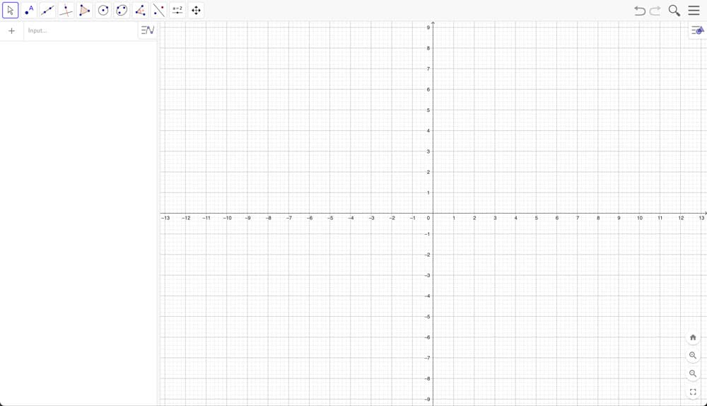
The interface for GeoGebra Classic 6 (almost identical to Classic 5 shown in the rest of this tutorial).

The first thing that I'd like to point out is that I am using GeoGebra Classic 5 - I love it. It does everything except 3D printing via STL files. You certainly could use the sixth version of it. I use Classic 5. They're almost identical.

Helpful hints when starting any GeoGebra script:

• Options: Turn off the labelling. Choose “no new objects”; otherwise, it gets very cluttered.
• Increase the font size.
• Choose the language of your choice; they even have Lithuanian!

There are really very few rules that you need to know in GeoGebra. It's a children's program to learn GEOmetry and alGEBRA. It’s simply wonderful.

First, let's get the basics down. The windows up on top are shown with different main icons. Below those are a series of drop-down sub-icons. We won't use all of these sub-menus, but we will use at least 25% of them all the time. So, remember that they're under the main windows on top.

Start with the Point icon, Fig 1, which is the first drop-down under the point window, and just drop down a few points.

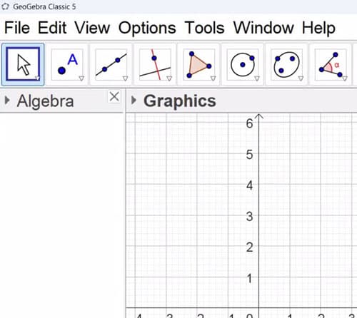
Fig 1. The Point tool to add a point to the canvas.

The exact location isn’t important. Immediately, you'll see the corresponding X and Y coordinates in the Algebra window on the left-hand side, Fig 2.

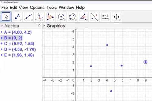
Fig 2. Points added to the 2D canvas and their coordinates in the Algebra window.

By default, we see the Algebra window to the left and the 2D geometry window to the right. There are other windows that you can access from the View menu, including a 3D view window. For now we’ll stick with the default windows.

Let's go to the segment menu and draw some segments between these points. The segment is under the third window from the left in Fig 3 below. Draw a few segments.

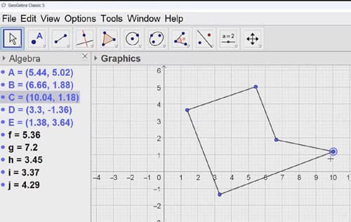
Fig 3. Line segments added between points on the 2D canvas.

Escape again, or click your mouse over to the big left Pointer icon on top, to get back to the pointer and notice what's happening now; things are tied together. Pull a point, and you will see the segments are dragged along with the point.

So now you can start to see this idea: that the segment depends on the points. The points are the parents, and the segments are the children. This next concept is kind of brutal. So brace yourselves.

If you kill the parent, you kill the children. What does that mean?

If you delete a point, its dependent children will disappear. To avoid this, hide it instead of deleting it. There are two ways to hide objects: right-click and select "show object" or use the hotkey button in the Algebra window to toggle visibility, Fig 4. Avoid deleting objects you don't want to see. Hide them to prevent screen clutter, which can happen quickly.

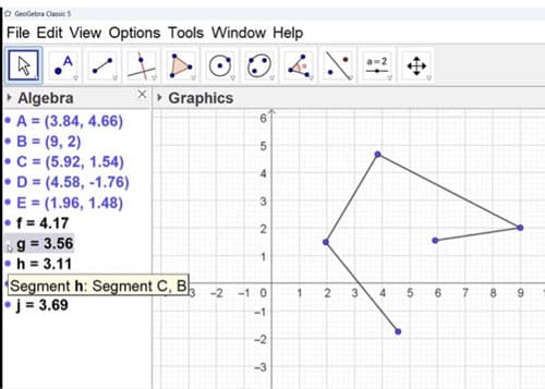
Fig 4. Toggle item visibility in the Algebra window.

The other thing I'd like you to notice is that this Algebra window is somewhat clumsily arranged. By default, new items show up in the order of their appearance. Click on the second toggle button below the word Algebra and go to that second menu. Do this to “sort objects by object type”, Fig 5. We will always sort objects by type in the Algebra window, not by the order of appearance.

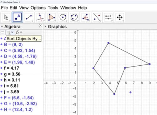
Fig 5. Sort objects by type in the Algebra window.

Parameterisation in GeoGebra

We want you to start designing in a parametric manner and to start to use parametric thinking. To explore parameterisation, let's set up a grid.

We will set up one point that is not parametric, and that will be point A1. Everything else will be built from this point. We call it A1 since this is where the grid line A and the grid line 1 intersect.

Now, here's the only rule that you really need to know in GeoGebra. Points begin with a capital letter.

So, let's manually type in A1=(0,0) into the input box and hit enter. We can see a new point on our canvas at location (0,0).

That's the only number that is locked or hardwired in. Everything else is parametric. Do not be tempted to hardwire a span or a load or an area. Put them in as variables, and use those variables in subsequent steps.

So, for instance, if I had spacing for my grid lines A, B and C, we should specify a SCALAR and call it spacingAB or spAB, Fig 6. Names of scalars do not require capital letters. Let's just say spAB is 7m, so spAB = 7. Spacing BC is 10m so in the Input bar type spBC = 10. And let's add one more spacing between gridlines C and D; for example let's say 8m, Fig. 6.

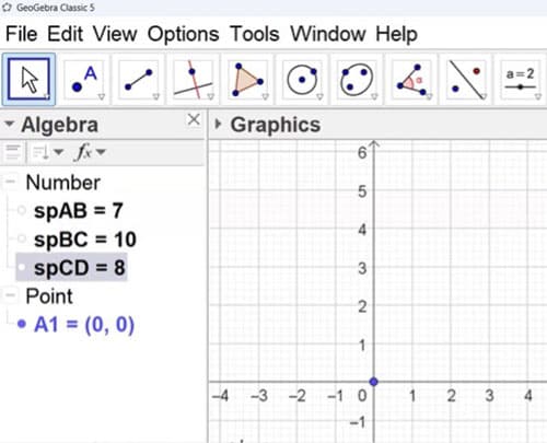
Fig 6. Defining parameters in the Algebra window.

Notice there are NO UNITS in GeoGebra, the user must be consistent with units. Notice also that variable names are CASE SENSITIVE, so if we say spCD = 8, we use the uppercase and lowercase letters to help us understand our own script and make it easy to read.

Always use the Input bar at the lower part of the screen for writing a single line of code. Most of it is perfectly intuitive, and there are prompts often to guide you on subsequent steps, much like Matlab or Python. If an item is grey, the program doesn’t know what you are referring to, if it is blue, the program knows what you are referring to.

Continuing with the grid line spacing, it is best to input subsequent Points parametrically. For example, add point A2 by typing A2 = A1 + (0, sp12). As we said already, do not hardwire or “hardcode” it in! Base it on previously established terms. This is the essence of parametric thinking.

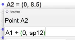
Fig 7. Add point A2 parametrically.

Similarly, other Points build off of previously established Points, Fig 8.

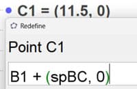
Fig 8. Add point C1 parametrically.

We could program all of the other gridline points in this manner. But there is a more efficient way. Use parallel and perpendicular lines to establish the other grid points. Parallel lines are located under the fourth menu window.

It is best to start by using the X axis or the Y axis and simply drop a parallel line through the points, Fig 9.

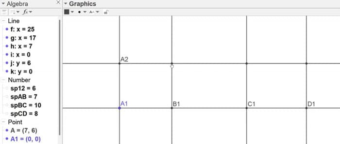
Fig 9. Establishing grid points using the parallel line tool.

If you can't find a particular item, just poke around and you'll quickly find it. But you could also think logically, what is the intersection of 2 lines? It's a point. So it's probably under the point menu. A quick look under the point, menu, and lo and behold, there's Intersect

The other fun thing is that you get to become really fussy about your drawings. My students are extremely fussy about their drawings, and I bet that you will become equally particular about how your drawings appear.

In the old days, we used to draw by hand and draftsmen (they were mostly men), but there must have been drafts women too, so let's call them draftspersons…they had their own style of drafting within the constraints of the building profession, but they were proud of their drawings!

You can personalise things here too. So, let's personalise the lines. Highlight all of the lines by just touching the main Line heading in the Algebra window, Fig 10. and all of the entities get highlighted.

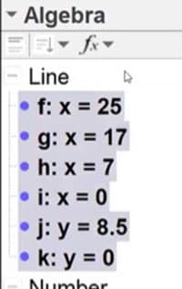
Fig 10. Highlighting all line entities in the Algebra window.

Right-click, and you can go to object properties and change the colour and the style of the lines. I prefer to do it using the hotkey on the graphics panel, Fig 11. You can select any properties you like, I’ve made the grid lines dashed green and reduced the line weight.

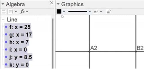
Fig 11. Changing the selected line properties using the interface hot-keys.

You can select your own style conventions but I’ve adopted the following; the grid lines are lightweight, beams are heavier, and girders are even heavier.