How I Coded an Analytical Beam Calculator

In this post, guest author Vittorio Lora talks us through how he developed the idea for and ultimately built Beamsolver.com. A structural engineer by training, Vittorio has pivoted in his career to focus more on software development. But he couldn’t shake the desire to build the analytical beam calculator that he would have found so helpful as a student. Parameterised structural analysis problems are notoriously difficult to solve algorithmically. Unlike numerical problems, solution techniques based on linear algebra just don’t scale well. Vittorio explains how it was actually the simple techniques we all learn first that ultimately unlocked the problem. Over to you Vittorio.

As a civil engineering student, I often found myself having to solve really complicated structures like this one,

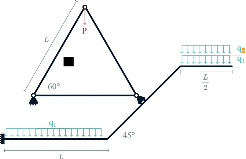
complicated-structure | EngineeringSkills.com

Fig 1. Complex parameterised structure.

I had to do it quickly and without errors. This was often just the first step in a much longer exam and a mistake here meant that everything else that followed would have been wrong as well! Those were fun times. If I wanted to have a chance to complete the test in time, I had to calculate the axial force, shear and bending moment of every beam in that structure in under fifteen minutes.

One key aspect of the structure above is that the beam lengths and the loads are symbolic quantities. This means that the diagram equations (axial force, shear and bending moment) are symbolic as well, since they are a function of those quantities. The regular FEA software that all engineers use can’t solve those kinds of problems, so I was out of luck if I wanted to check whether my results were correct or not.

The lack of a program that could do this is what ultimately pushed me to code Beamsolver, an online beam and frame calculator that lets the user find the analytical solution of both determinate and indeterminate structures.

Try Beamsolver today, completely free.

A little bit about me

My name is Vittorio and I have studied Structural Engineering at the university of Trento, Italy. Even though nowadays I focus more on software development than anything else, I still have a passion for civil and structural engineering. I enjoy writing software that solves real problems and makes people’s life easier.

1.0 The need for an analytical beam calculator

When engineers have to do structural analysis (i.e. finding the internal forces of beams, trusses, etc.) they often use Finite Element Analysis (FEA) software to help them with the calculations. There are hundreds of programs that can do that, some of which are completely online.

Using the Finite Element Method, you can find an approximation of the internal forces, but you can’t find the actual analytical equations. The problem is that FEA analysis requires numerical quantities as inputs, so if you are trying to calculate the actual equation of the maximum bending moment in the first beam of the following configuration you are out of luck,

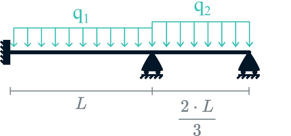
double-span-beam | EngineeringSkills.com

Fig 2. Parameterised multi-span indeterminate structure.

But why bother with the analytical solution if real-world quantities are always numerical? Well, knowing the equations of the internal forces can often be really helpful. They open up the possibility for powerful parameter-driven design, and are much more versatile to implement. For example, once you know the bending moment equation for the above configuration, that equation is valid for any beam length and load value, if we assume the behaviour of the structure remains linear. Very useful if you have to design a lot of similar beams!

It’s also very useful to engineering students who are learning structural analysis. The ability to see the actual formula is much more insightful than a numerical value in $kNm$ .

For those who are interested, the formula of the bending moment in the first beam is:

M\left(s_0\right)=-\cfrac{q_{1}\cdot s_{0}^{2}}{2}+\cfrac{19\cdot L_{}\cdot q_{1}\cdot s_{0}}{34}+\cfrac{2\cdot L_{}^{2}\cdot q_{2}}{153}-\cfrac{2\cdot L_{}\cdot q_{2}\cdot s_{0}}{51}-\cfrac{7\cdot L_{}^{2}\cdot q_{1}}{68}

Where $s_0$ is the axial coordinate along the beam.

1.1 Drawbacks and practical limitations of an analytical approach

The problem with trying to find the analytical solution is that some structures are just too complicated, and the equations become so big that it would be pointless to calculate them. In those situations it’s better to stick to numerical values. This is often the case for structures where the geometry is very complicated, or for highly indeterminate configurations where both bending deformation and axial deformation need to be taken into account.

2.0 Why finding the analytical solution is difficult

So, the goal for me was to write a programme capable of finding the analytical solution. I wanted to code an application that could run online, that would allow the user to draw a structure through a nice user interface (UI) and display the results as nicely formatted formulas and diagrams.

I soon realised why an application like this didn’t exist: symbolic computation can be very complicated, is notoriously slow, and is difficult to generalise. I needed basically two elements to make this feasible:

A Computer Algebra System (CAS): This is the part of the code that deals with symbolic computation. It can run algebraic calculations with variables, get integrals and derivatives, etc;
A general algorithm to solve determinate and indeterminate structures: This is the algorithm that, given a structure of beam or trusses as input, finds the support reactions and the internal forces using the computer algebra system to keep everything symbolic.

Because I was familiar with python, I decided I would use sympy (a python library) as my CAS of choice. With that sorted, all I had to do was write the algorithm.

2.1 Inverting a symbolic stiffness matrix

My first idea was to simply write a regular FEM software in python, but use sympy to keep everything symbolic. The finite element method is just a way to discretise a problem into a set of linear equations, generally written like this:

\mathbf{K}\cdot x=b

In structural engineering, the matrix $\mathbf{K}$ is called the stiffness matrix. All I had to do was to calculate the stiffness matrix using sympy, and then invert it to find the analytical solution, just like in a regular finite element analysis program.

This approach worked fine, provided that the structure had only one beam. Anything more than that and finding the inverse stiffness matrix took exponentially longer. I was forced to abandon that idea and start thinking outside of the box.

When I had to solve complicated structures for my university exams, I didn’t use a stiffness matrix. I used regular old free-body diagrams and equilibrium equations. I realised that maybe I could write an algorithm that did something similar, finding the system of equilibrium equations and solving it using the computer algebra system.

3.0 The general approach to solving structures analytically

I had to come up with a way to write the equilibrium equations reliably for every beam configuration a user could think of. The first question I asked myself was: what are the unknowns of this problem? In other words, what am I actually trying to calculate?

Well, my goal was to find the equations of the internal forces (axial force, shear and bending moment) along any given beam of the input structure. That is pretty easy to do using the method of sections, once you know the forces acting at the two ends of every beam. The first thing I did was define a sign convention:

Fig 3. Sign convention for axial force $N$ , shear force $V$ and bending moment, $M$ .

The values of $N$ , $V$ and $M$ at the end of every beam are the unknowns of the problem. Beams are connected together by nodes, in which we find the same unknowns plus the support reactions. Perhaps the best way to understand this is to draw the “exploded” diagram of a structure:

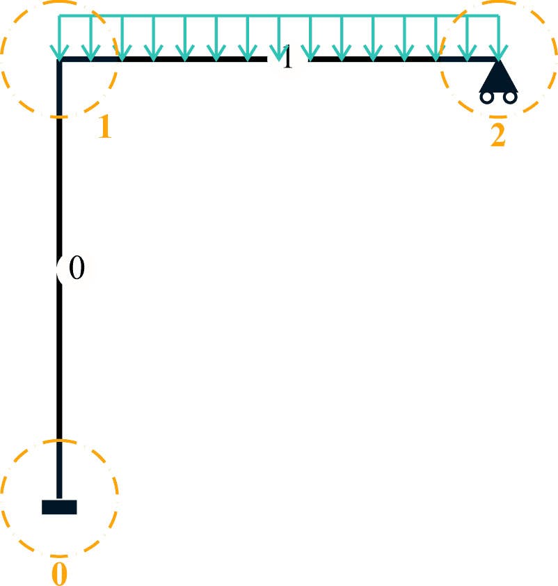
Fig 4. Indeterminate frame structure indicating nodes $0$ , $1$ and $2$ .

We will use this structure as an example throughout this explanation. It helps to visualise the forces in an “exploded” diagram:

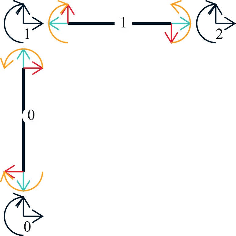
exploded frame example | EngineeringSkills.com

Fig 5. ‘Exploded’ frame revealing the internal actions at the nodes.

The dark arrows represent the support reactions, and the colourful arrows represent the values for $N$ , $V$ and $M$ at the ends of every beam.

This is the free-body diagram of the structure, and all equilibrium equations are written with this diagram in mind. For every node $j$ connected to a beam $i$ , we can write the internal forces as

N_{i,j},V_{i,j},M_{i,j}

We also need a naming convention for the support reactions. Given a node $j$ we can write

R_{j,h},R_{j,v},R_{j,r}

In the example above there are 21 unknowns, which means that we need 21 equations in order to have a closed solution. If we were solving the structure above by hand, we would be a little smarter than this and not even bother to include, say, $R_{2,h}$ because it is obviously equal to zero. However, in the context of writing a computer algorithm, it’s much better to include everything and then simply add an additional $R_{2,h}=0$ equation to the system.

So once I understood how to discretise the structure with this approach, the next step was to write the equilibrium equations. There are two types of entities in the diagrams: nodes and beams. Equilibrium equations can be written for both, let’s see how.

3.1 Beam equilibrium equations

For a beam laying on a 2d plane, we can write two translational equations and one rotational equation. The general configuration looks something like this:

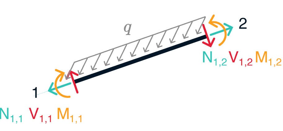
beam-equations-general | EngineeringSkills.com

Fig 6. General parameterisation of a beam element.

The beam is at an arbitrary angle with respect to the horizontal axis, and the distributed load is at an arbitrary angle with respect to the beam. I will spare you the general equations, but as you can imagine there is a lot of trigonometry involved here. On top of this, the distributed load (of which there can be more than one!) can be trapezoidal, further complicating matters.

One important thing to note here is that there can not be discontinuous sections along the beam. This means no point loads and no abrupt changes to the distributed load. In order to deal with such configurations it is much easier to simply split the beam into multiple chunks, connected together by continuous nodes, and write the free body diagram of each additional chunk and node separately. This also ensures that all the point loads applied to the structure only appear inside the node equilibrium equations, and not the beam equilibrium equations.

We get the following equations for the two beams of our structure:

Beam 0

\begin{cases} N_{1,0}-N_{0,0}=0\\ V_{0,0}-V_{1,0}=0\\ M_{0,0}-M_{1,0}+L_{}\cdot V_{1,0}=0 \end{cases}

Beam 1

\begin{cases} N_{2,1}-N_{1,1}=0\\ V_{1,1}-L_{}\cdot q_{}-V_{2,1}=0\\ M_{1,1}-M_{2,1}+\cfrac{L_{}^{2}\cdot q_{}}{2}+L_{}\cdot V_{2,1}=0 \end{cases}

3.2 Node equilibrium equations

Nodes also have two translational equations and one rotational equation. The same internal forces that we used to write the equilibrium equations of the beams appear here as well, except they are flipped.

Nodes are where the structure is attached to the ground, so the support reactions are also going to be part of the equations.

The general configuration looks something like this:

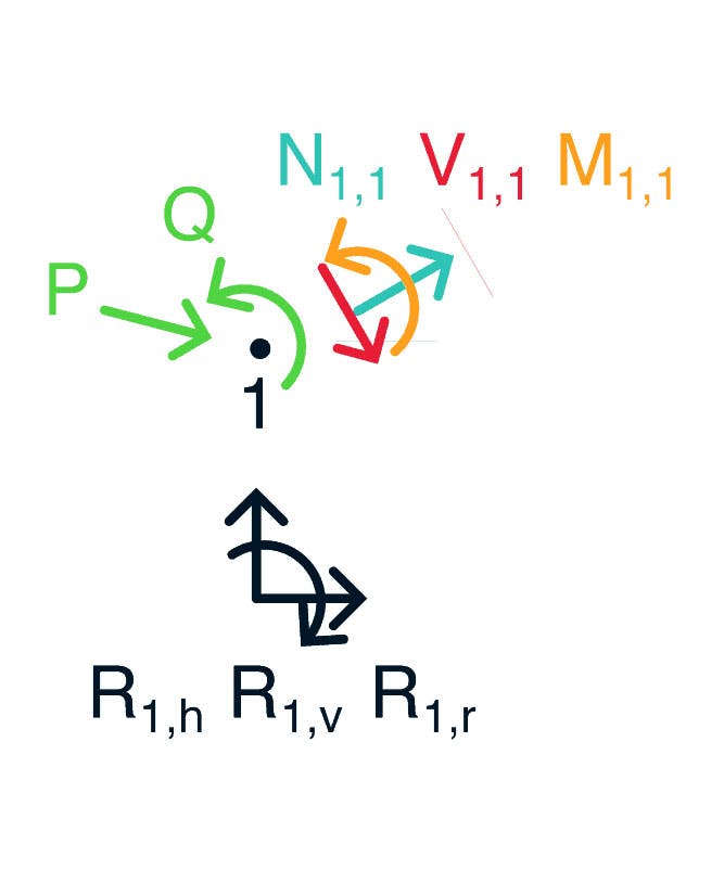
Fig 7. General parameterisation of a node.

There can be $n$ beams converging into a joint at arbitrary angles. Point loads also are applied at arbitrary angles, and if support reactions are present, they could be rotated as well (like in the case of a vertical roller at a 30° angle). Again, I will spare you the general equations.

On top of the three equilibrium equations of the free-body diagram, we have to also take into consideration the type of support and hinge a particular node has. This allows us to write more equations by setting some of the reactions or some of the internal forces equal to zero, in accordance with the node type.

There are a lot of possible combinations, and describing all of them goes beyond the scope of this article. The key takeaway here is that by adding these equations we are “inserting” the information about the boundary conditions into our final system.

Here are the equations for the three nodes in the example structure.

Node 0

\begin{cases} R_{0,h}+V_{0,0}=0\\ N_{0,0}+R_{0,v}=0\\ R_{0,m}-M_{0,0}=0 \end{cases}

Node 1

\begin{cases} N_{1,1}+R_{1,h}-V_{1,0}=0\\ R_{1,v}-N_{1,0}-V_{1,1}=0\\ M_{1,0}+R_{1,m}-M_{1,1}=0\\ +R_{1,h}=0\\+R_{1,v}=0\\ +R_{1,m}=0 \end{cases}

Node 2

\begin{cases} R_{2,h}-N_{2,1}=0\\ R_{2,v}+V_{2,1}=0\\ M_{2,1}+R_{2,m}=0\\ +R_{2,h}=0\\ +R_{2,m}=0 \end{cases}

3.3 Solving the system of equilibrium equations

Once I managed to write the code that generated the system of equations, the next step was to solve it. One thing to note here is that I made no distinction between determinate and indeterminate structures: the system could have more variables than equations, and that was ok. This means that sometimes the solution would contain some of the unsolved variables. These could then be calculated using the principle of virtual work, but more on that later.

So I had this symbolic linear system that I needed to solve. To make a long story short, I had to implement my own specialised algorithm, because the functions that came with the CAS I was using at the time were too slow. I implemented the method of backward substitution:

solve the last equation of the system for the first variable found in that equation;
substitute the result in the other equations;
do the same for all the other equations, going backwards.

If the structure that generated the system was determinate, I would get a closed solution. If it was indeterminate, the solution would contain leftover variables.

Solving the system for our example structure, we get the following result:

\begin{cases} N_{0,0}=R_{2,v}-L_{}\cdot q_{}\\ V_{0,0}=-0\\ M_{0,0}=-\cfrac{L_{}^{2}\cdot q_{}}{2}+L_{}\cdot R_{2,v}\\ N_{1,0}=R_{2,v}-L_{}\cdot q_{}\\ V_{1,0}=-0\\ M_{1,0}=-\cfrac{L_{}^{2}\cdot q_{}}{2}+L_{}\cdot R_{2,v}\\ N_{1,1}=-0\\ V_{1,1}=-R_{2,v}+L_{}\cdot q_{}\\ M_{1,1}=-\cfrac{L_{}^{2}\cdot q_{}}{2}+L_{}\cdot R_{2,v}\\ N_{2,1}=-0\\ V_{2,1}=-R_{2,v}\\ M_{2,1}=-0 \end{cases}

Note the presence of $R_{2,v}$ in the solution. This leftover variable tells us that this structure has one degree of indeterminacy. In order to calculate it, we need to apply the Principle of Virtual Work, but before we can do that we need to get the equations of the internal forces.

3.4 Getting the axial force, shear and moment diagram equations

It was pretty easy to write the code that calculated the diagram equations by method of sections, since the solution of the system gives us the values of the diagrams at the ends of every beam.

For our specific example, we get the following equations:

Equations for beam 0:

\begin{cases} N\left(s_{0}\right)=R_{2,v}-L_{}\cdot q_{}\\ V\left(s_{0}\right)=-0\\ M\left(s_{0}\right)=-\cfrac{L_{}^{2}\cdot q_{}}{2}+L_{}\cdot R_{2,v}\\ \end{cases}

Equations for beam 1:

\begin{cases} N\left(s_{1}\right)=-0\\ V\left(s_{1}\right)=-R_{2,v}-q_{}\cdot s_{1}+L_{}\cdot q_{}\\ M\left(s_{1}\right)=-R_{2,v}\cdot s_{1}-\cfrac{L_{}^{2}\cdot q_{}}{2}-\cfrac{q_{}\cdot s_{1}^{2}}{2}+L_{}\cdot R_{2,v}+L_{}\cdot q_{}\cdot s_{1}\\ \end{cases}

3.5 Principle of Virtual Work

In the case of indeterminate structures, the equilibrium equations are not enough. We need additional equations to get rid of the leftover variables from the solution. For Beamsolver, I found that using the principle of virtual work was the easiest way to get around this problem.

I will not go in-depth on the principle of virtual work, but in general for every indeterminate unknown $X_{i}$ you can write the following equation:

\sum_{j=0}^{n}\cfrac{1}{E_j\cdot A_j}\cdot \int\limits_{0}^{L_j}N\cdot \cfrac{\partial N}{\partial X_i}ds_j+\sum_{j=0}^{n}\cfrac{1}{E_j\cdot J_j}\cdot \int\limits_{0}^{L_j}M\cdot \cfrac{\partial M}{\partial X_i}ds_j

Where $j$ indicates a beam of the structure. Most of the time, people don’t take the axial deformation into account, so the term with $E_{j}\cdot A_{j}$ disappears. This makes calculations considerably simpler, because you can then simplify the term $E \cdot J$ from the final equation (provided that all beams have the same section properties).

Our example only has one indeterminate variable, so the principle of virtual work gives us only one additional equation:

-\cfrac{5\cdot L_{}^{4}\cdot q_{}}{8\cdot E_{}\cdot J_{}}+\cfrac{4\cdot L_{}^{3}\cdot R_{2,v}}{3\cdot E_{}\cdot J_{}}=0

Solving for $R_{2, v}$ we get:

R_{2,v}=+\cfrac{15\cdot L_{}\cdot q_{}}{32}

We can then substitute this result in the equations of the diagrams to get the final solution.
For beam 0:

\begin{cases} N\left(s_{0}\right)=-\cfrac{17\cdot L_{}\cdot q_{}}{32}\\ V\left(s_{0}\right)=-0\\ M\left(s_{0}\right)=-\cfrac{L_{}^{2}\cdot q_{}}{32} \end{cases}

For beam 1:

\begin{cases} N\left(s_{1}\right)=-0\\ V\left(s_{1}\right)=-q_{}\cdot s_{1}+\cfrac{17\cdot L_{}\cdot q_{}}{32}\\ M\left(s_{1}\right)=-\cfrac{q_{}\cdot s_{1}^{2}}{2}-\cfrac{L_{}^{2}\cdot q_{}}{32}+\cfrac{17\cdot L_{}\cdot q_{}\cdot s_{1}}{32} \end{cases}

And there you have it, those are the equations of the internal forces. This is the general method I currently use in Beamsolver to solve basically every possible structure configuration imaginable. Nothing revolutionary really, just solve the equilibrium equations and use virtual work when needed. The challenge for me was to translate all of this into code, which is what the next part of this article will focus on.

4.0 The first version of Beamsolver

The very first time I started to tinker with the idea of an analytical beam calculator was back in my third year of university, when I had to do my solid mechanics exam. I had a really cool graphing calculator from Texas Instruments that came with a built-in computer algebra system, so I started writing a simpler version of the algorithm I described above (it only worked for determinate structures) that would run on the calculator.

I put in a lot of hours over about three weeks, and then one day my computer crashed while I was coding. When I rebooted, good news! My project files were still there. Except they all had a size of 0Kb. Being a naive and inexperienced programmer, I didn’t have any backups, so I lost all my work. Always save your work on the cloud folks.

As a student I was very busy, and never found the time to re-write the code I had lost. But the idea was still there in the back of my head, and I finally got the chance to attempt this project again a couple of years later.

This is where the python experimentation I talked about started. By that time I had become a much better programmer, and was confident I could do it. My goal was to create a web application that people could use from all over the world.

While I was a good python programmer, I had absolutely no idea how the web worked, let alone how to create a full blown web application. I did a lot of learning over the course of a couple of weeks, and came to the conclusion that if I were to do this, python was not the right choice.

The problem with python was that it can only run in a server, and not in a browser. This meant that while I could write the algorithm I wanted, I would have to pay for a pretty beefy server setup, especially if I got a lot of users.

4.1 Moving away from Python

Thus began my journey in the world of Javascript. My goal was to write something that would run entirely client-side, meaning basically zero load on my server. I went on a coding frenzy for a month and a half, learned a lot, and finally put the first version of Beamsolver online during the summer of 2020. At the time it was called SylBeam, and it had limited functionality, but it worked.

I was so exhausted after that coding sprint that I didn’t have the strength to add the features that were missing, or to do any kind of marketing. I also had to start studying again for my exams, so my time became very limited. SylBeam remained online, but I ended up putting the project on the sidelines for another two and a half years.

5.0 Making a serious commitment, and the current version of Beamsolver

I graduated at the end of 2020, and was immediately caught in a whirlpool of different projects and opportunities. I never had a real job since I’m more of a freelance/entrepreneur kind of guy, and I made the choice to focus more on my programming skills than my potential career as a structural engineer, which I completely abandoned.

Having said that, I absolutely hate leaving a project unfinished. I knew the potential that Beamsolver (which at the time was still called SylBeam) had. I now had the skills to not only execute the idea the way I wanted, but to turn it into a business as well. I took a two week break from everything to go take a sailing course, and when I came back I felt inspired enough to get on with it.

5.1 Starting from zero one last time

After taking a quick look at the spaghetti code I had written years before, I decided to re-do everything from scratch. The biggest problem with javascript is that it doesn’t have a good CAS library like python. For SylBeam, I had to use three separate computer algebra systems in tandem, because none did all the things I needed correctly. That kind of approach was simply not up to production standards.

5.2 Writing a computer algebra system from scratch

I knew I had to write my own CAS in javascript. That was the biggest challenge that kept me from completing this project during all those years. I knew I could do it, but man was it difficult. Of the two and a half months it took me to finally push the app into production, more than half was spent getting the computer algebra system to work. I ended up calling it SylCas, in honor of the first version of Beamsolver.

Doing it myself came with a big advantage. I could tailor it to do exactly what I needed and nothing more, which allowed me to make it fast. It still can’t solve every structure imaginable, but that’s ok. The formulas for those configurations are so huge that they become pointless.

The good news is that I wrote it so it could handle numerical computations as well, so for those problems that are unsolvable analytically it can still find a solution, provided you give numerical inputs like you would do for a regular FEM software. After all, the general algorithm I described in this article works just as well with numeric values as it does with symbolic ones.

I could probably write an entire book on the computer algebra system alone, it was such a complex undertaking. For this article, this brief paragraph will have to do.

6.0 Coding the UI and Putting it all Together

The final step before I could launch the app was to code a nice user interface that would allow the users to quickly draw the structure they wanted, click a button to solve it, and explore the solution. My philosophy when it comes to UI is less is more. The more stuff you add, the more stuff that can go wrong!

In general, here is the functionality I wanted to include:

A diagram of the structure, with all the loads and supports;
An input menu where the user would specify the properties of the various elements of the structure, such as support types, beam lengths, section properties and so on;
The $N$ , $V$ , $M$ diagrams of the solved structure;
The formulas of the internal forces of the solved structure, with the ability to calculate derivatives, inflection points, maximum values and so on;
A step-by-step version of all the calculations made to find the solution.

It took me a couple of weeks of tinkering to get something that looked nice, but in the end I was quite proud of the result I got. Here are some screenshots:

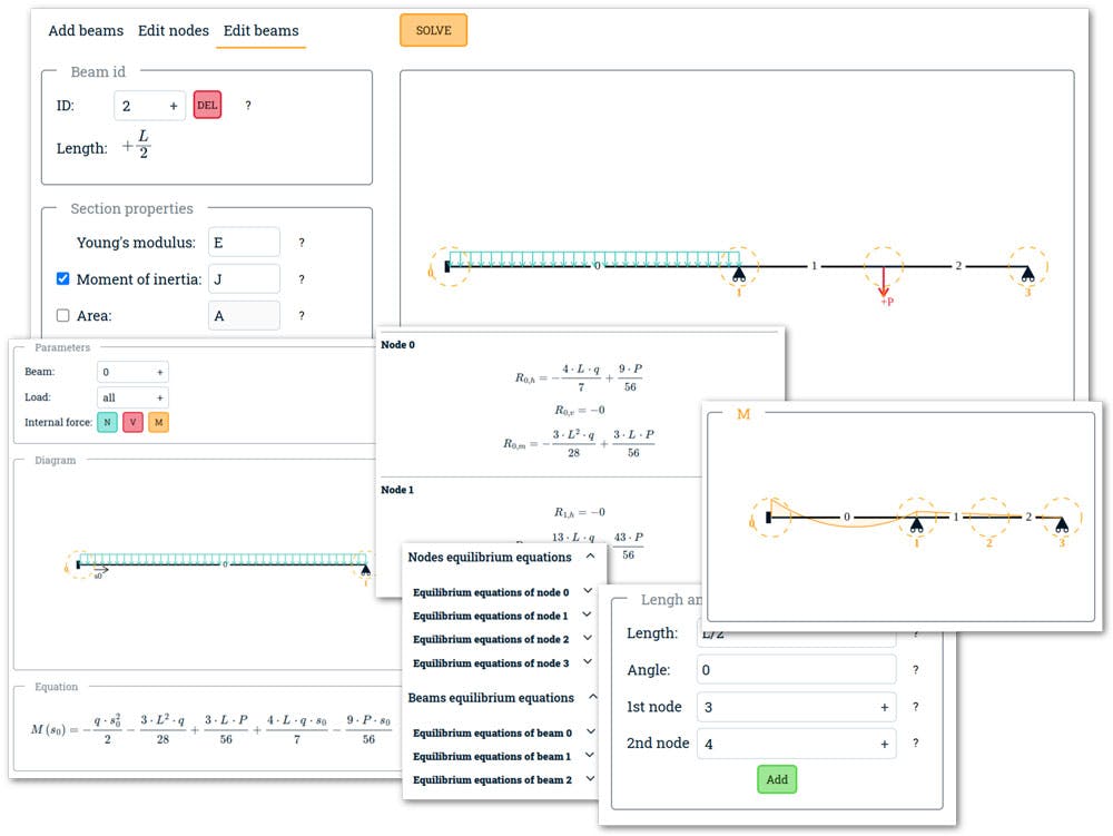
Beamsolver screenshots | EngineeringSkills.com

Fig 8. Beamsolver user interface screenshots.

Once I had a working UI, the app was basically done. All I had to do then was build a website around it, allow users to register, set up a payment provider, and in general all the stuff that a full-stack developer does to push something into production. I’m really glad I finally managed to complete (well, sort of) this project, after almost five years since I first envisioned it.

7.0 What’s next for Beamsolver?

Appetite comes with eating, and now that I’m done I have more ideas I want to implement. Some are just small add-ons that should have been included from the beginning, like deflection equations, load combinations, and better mouse interaction. Others would take a bit more time. For example I really want to publish the computer algebra system I wrote as a free library, but I just never have the time to do it.

I also want to expand Beamsolver by adding support for a section designer (with symbolic quantities, of course!), the ability to make design decisions according to codes, a way to export the results in a nicely formatted pdf file, the list goes on.

It was only by writing this article that I realized how long I had been working on this project. The idea for Beamsolver has accompanied me through most of my years as a student, and has been a huge catalyst in my journey as a programmer. The knowledge I gained while trying to solve this problem has truly reshaped my career, and has given me access to some amazing opportunities.

If you are interested in programming as well, my advice to you is to find some kind of problem that sparks your interest, and try to write some code to solve it. This is much more effective than just learning to code for the sake of it by watching tutorials. You need a catalyst to drive you, otherwise it just becomes another thing you have to study!