An Introduction to form-finding with Thrust Network Analysis
![[object Object]](/_next/image?url=%2Fimages%2Fauthors%2Foliviero_cabitza.jpg&w=256&q=75)
In this tutorial, Oliviero Cabitza provides an excellent deep dive into Thrust Network Analysis, a powerful form-finding method for compression-only masonry vaults and shell structures. Thrust network analysis is an exciting and relatively new method of form-finding and something I've been looking forward to turning my attention to. I'm delighted that Oliviero, a long standing member of the EngineeringSkills community has stepped forward to share his knowledge.
From my correspondence with Oliviero on the topic, I know that he's been putting this technique to good use and I'm looking forward to him sharing more on the topic in future tutorials - but for now, let's get the basics under our belt!
Starting from the elegant simplicity of Hooke's hanging chain and working through graphic statics and Heyman's safe theorem, Oliviero takes us through the full mathematical framework of TNA as developed by Philippe Block.
Whether you're interested in the assessment of existing masonry structures or the design of new funicular shells, Thrust Network Analysis provides a rigorous and intuitive approach. This is a great introduction to the topic of form-finding and using thrust network analysis.

1. What is Thrust Network Analysis?
Thrust Network Analysis (TNA) is a form-finding method particularly suited to any type of vaulted structure made of unreinforced masonry. This method can be applied both to the assessment of existing masonry vaults and to the exploration of possible equilibrium solutions for funicular shells.
Developed by Philippe Block in his 2009 PhD thesis, TNA extends the principles of Thrust Line Analysis (TLA) - traditionally used to verify the stability of arches, into three dimensions, making it applicable to vaults and shell structures. Before diving into how TNA works, it is useful to first recall the three key concepts that made its development possible.
1.1 Hooke's Hanging Chain
The first of these concepts is Hooke's hanging chain principle, also known as Hooke's law of inversion. Robert Hooke (1635 - 1703) was one of the most important scientists of the 17th century. In 1676 he published ten "Inventions" in the form of anagrams. The third of these inventions was
ceiiinosssttuv
whose solution, published later, was
Ut tensio, sic vis
Latin for "As the extension, so the force". This is Hooke's law of elasticity, which earned him a place among the founders of modern structural mechanics. However, in this article we are more interested in his second invention
2. The true Mathematical and Mechanical form of all manner of Arches for Building, with the true abutment necessary to each of them. A Problem which no Architectonick Writer hath ever yet attempted, much less performed.
abcccddeeeeefggiiiiiiiillmmmmnnnnnooprrsssttttttuuuuuuuux
Its solution, published after Hooke's death, reads
Ut pendet continuum flexile, sic stabit contiguum rigidum inversum
In English:
As hangs the flexible line, so but inverted will stand the rigid arch

Fig 1. The first five of the ten 'Inventions' of Robert Hooke (from British Society for the History of Mathematics).
The idea is powerful in its simplicity: the shape of a hanging chain, which carries only tension, if frozen and inverted, defines the geometry of a purely compressed arch. The hanging model can be composed of discrete weights proportional to the voussoirs' self-weight, connected by a rope of negligible weight. When inverted, this produces a thrust line that fits within the thickness of the arch.
This concept was later applied by the mathematician and physicist Giovanni Poleni in 1743, when assessing the stability of St. Peter's Dome. Two centuries after its completion, several cracks had appeared, but Poleni observed that they had effectively divided the dome into fifty arches sharing a common keystone. By verifying that the inverted chain lay entirely within the masonry, he demonstrated the dome's stability—showing that as long as the thrust line remains within the material, the arch (and thus the vault) is stable, even when cracked.

Fig 2. On the left, Hooke's hanging chain and the corresponding inverted compressed arch; On the right, Giovanni Poleni's analysis of the dome of St Peter's in Rome using Hooke's hanging chain principle (from Poleni, 1747).
1.2 Graphic statics
Instead of using a hanging model, graphic statics can be applied for two-dimensional structures. Given the external loads, graphic statics makes it possible to determine both the possible funicular shapes and the magnitude of internal forces. (For further insight, see this article by Prof. Edmond Saliklis, which explains how graphic statics works and illustrates the technique through a truss example.)
Consider the arch composed of irregular voussoirs shown in Figure 3(a). Each voussoir has a self-weight, represented by a concentrated force of proportional magnitude applied at its centroid. Each of these forces acts along a vertical line of action.
Each voussoir is held in place by the compressive forces exchanged with its adjacent blocks, as depicted in Figure 3(c). In this way, the load is transmitted down to the supports through compression. The equilibrium of a single voussoir can be represented by a closed polygon (a triangle), as shown in Figure 3(d). The overall force polygon is then composed of the triangles corresponding to the equilibrium of each voussoir, as represented in Figure 3(b).
From the force polygon we can observe that the two sides, Foa and Foh, represent the reactions at the spring points. These are the forces with the greatest magnitudes, indicating higher compressive stresses near the supports. Conversely, at the keystone (W4) the compressive forces reach their minimum values.
It is worth noting that an infinite number of funicular polygons - or thrust lines, can be drawn within the thickness of the arch. The geometry of each thrust line depends on the length of the equivalent chain and the horizontal distance between the supports. Many different thrust lines can, therefore, exist between the extrados and the intrados of the arch.
In other words, the structure is statically indeterminate: multiple equilibrium solutions are possible. But what can we do with this information if we do not know which one corresponds to the actual thrust line?

Fig 3. For a random arched structure, (a) a possible thrust line and its equivalent hanging chain are constructed using graphic statics; (b) the force equilibrium of the system is represented in the funicular polygon; (c) the equilibrium of one of the voussoirs; and, (d) the vectors representing the forces in and on the block (Block, DeJong and Ochsendorf, 2007).
1.3 Heyman's Safe Theorem for Masonry
Claude-Louis Navier (1785–1826) was another of the founders of modern structural mechanics. He argued that engineers, or anyone wishing to assess the stability of a structure, should be primarily concerned with the calculation of stresses within its elements.
To determine the stress state inside a structure, one must first evaluate the internal forces. This starts with solving the equilibrium equations, which is only straightforward when the structure is statically determinate (typically the case for isostatic systems).
If the structure is statically indeterminate (hyperstatic), determining the internal stresses requires adopting an elastic constitutive law together with specific boundary conditions (for example, at the abutments of an arch). Both of these are approximations of reality: the material response is not perfectly elastic (or only within a limited range), and it is difficult to define an "exact" stress–strain law for an assemblage of stone and mortar. Moreover, even small changes in boundary conditions, such as minor settlements at supports assumed to be fixed, can lead to a different elastic solution (that is, a different position of the thrust line).
In other words, the "exact" solution — the actual stress state within the masonry — is a chimera, something we can define in theory but never truly capture in practice.
What has just been outlined is usually referred to as elastic theory. However, the following experimental observation led to what is known as plastic theory: if several seemingly identical structures, each with small imperfections and thus different initial internal stress states, are slowly loaded to collapse, they will be found to fail at essentially the same load. The key requirement for the application of plastic theory is that collapse occurs through a ductile, quasi-static process; plastic theory is therefore not directly applicable to brittle materials.
To apply plastic theory, one must examine the possible mechanisms by which a structure might collapse. The fundamental safe theorem of plasticity states that, if an equilibrium state can be found in which the internal forces are in balance with the external loads and every part of the structure satisfies a given strength criterion, then the structure is safe under those loads.
Jacques Heyman (born 1925), professor at the University of Cambridge, formulated an analogous safe theorem for masonry structures. His approach requires three key assumptions in order to analyse masonry within the framework of plastic theory:
- masonry has no tensile strength;
- stresses are sufficiently low that masonry can be considered to have unlimited compressive strength;
- sliding failure cannot occur.
The master "safe" theorem for masonry states that, if the previous conditions are satisfied:
If a position of the thrust line can be found for it to lie within the masonry, this is a proof that the structure is stable and indeed that collapse can never occur under the given load.
The thrust line, or funicular polygon (Hooke's inverted chain), represents the condition of equilibrium. If it lies within the masonry, only compressive stresses are present, which satisfies the first assumption. Note that although individual stones may possess some tensile strength, the mortar between them is typically very weak in tension.
Regarding the second assumption, it can be considered approximately valid when average stress levels are examined. In historic masonry, the average compressive stresses are often two orders of magnitude lower than the compressive strength of the stone, due to the large structural depth. Local stress concentrations may develop and cause limited damage, but they do not usually lead to global structural failure.
As for sliding failure, it is observed that, although local slippage of individual blocks may occur, masonry structures generally retain their overall shape. This implies that a modest level of compressive prestress is often sufficient to prevent significant sliding and a general loss of cohesion.
1.4 From Thrust Line Analysis to Thrust Network Analysis
Heyman's safe theorem tells us that a masonry structure is safe if we can find at least one admissible thrust line entirely contained within its thickness, in equilibrium with the applied loads. This is precisely what Thrust Line Analysis (TLA) achieves: using graphic statics to generate thrust lines that visualise the possible compressive force paths through the structure.
TLA's main limitation, however, is that it applies only to two-dimensional problems. Fortunately, the concepts we have just explored can be extended to three dimensions.
Just as Hooke's hanging chain principle was used historically to study and verify the stability of arches—and later extended to axially symmetric domes—three-dimensional hanging models have been employed to design complex vaulted shells. The Catalan architect Antoni Gaudí (1852–1926) famously used models made of strings and weights to explore the shapes of some of his masterpieces, such as the Sagrada Família (see Figure 4). Later, architects and engineers like Heinz Isler (1926–2009) and Frei Otto (1925–2015) applied similar hanging models to design innovative shell structures.

Fig 4. Gaudí's hanging model of Sagrada Familia (from List of Physical Visualizations and Related Artifacts).

Fig 5. Frei Otto's hanging chain model for the Mannheim Multihalle (Liddell, 2015).
Although physical models were (and still are) valuable tools during the conceptual design phase, modern numerical form-finding procedures are far more convenient. As we have seen, instead of using a hanging chain, one can draw a thrust line using graphic statics.
Similarly, Thrust Network Analysis (TNA) replaces three-dimensional hanging models, enabling the exploration of compression-only shell structures. A thrust network is simply the three-dimensional counterpart of a thrust line: just as the latter represents one possible state of static equilibrium in compression under given loads, so does the former — and Heyman's safe theorem applies in both cases.
TNA considers only vertical loads (typically self-weight). While this is a significant simplification, it allows the form-finding process to be split into two distinct steps:
- First, horizontal equilibrium is established for the thrust network; this requires only its plan geometry and boundary conditions (restraints);
- Then, vertical equilibrium is solved, determining the heights of the network nodes based on the boundary conditions, vertical loads, and the horizontal force state from step one.
This assumption of purely vertical loads is well-suited to vaults where self-weight dominates. Figure 6 illustrates the relationship between the thrust network G, its horizontal projection, the form diagram , and the force diagram — the reciprocal dual of .

Fig 6. Relationship between the thrust network (G), its planar projection, the form diagram and the reciprocal force diagram (Block, 2009).
In the next section, we will explore how the thrust network, force diagram, and form diagram interrelate, along with the mathematical formulation and computational process behind this form-finding methodology.
2. How does TNA work?
2.1 The relationship between thrust network, form diagram and force diagram
At the end of the previous section, we have seen that the form diagram represents the horizontal projection of the thrust network G, while the force diagram allows us to compute the equilibrium of , that is, the horizontal equilibrium of G. The branches of the force diagram represent the forces in the corresponding edges of the form diagram (i.e., the horizontal projection of the forces in the thrust diagram). This means that corresponding edges in and must be parallel, as only axial forces are allowed.
In fact, and are reciprocal dual graphs: branches that come together at one node of one diagram form a closed polygon in the other, and vice versa (Figure 7). From a structural point of view, this property ensures equilibrium. Furthermore, when the closed polygons of (which represent the equilibrium of the corresponding nodes of ) are all oriented clockwise, both and G will be in compression.

Fig 7. Reciprocal relationship between the form diagram and the reciprocal force diagram (Block, 2009).
Notice that for a given form diagram , several force diagrams can be drawn that satisfy the condition that corresponding branches are parallel. For a three-valent form diagram, i.e., a form diagram in which three branches converge at each internal node (Figure 7), we have only one degree of freedom, corresponding to the possibility of scaling the diagram: a larger force diagram - that is, one with longer branches, corresponds to greater horizontal thrusts, which are associated with shallower thrust networks G (as arches with smaller depths have greater horizontal thrusts).
Hence, a three-valent form diagram is structurally determinate up to a scale factor. This means that it is not possible to redistribute the internal forces within these networks. This does not apply when the form diagram has nodes with valences higher than three: in this case, we can find different force diagrams, all in equilibrium with the same form diagram, but where branches can vary locally in length (i.e., not necessarily by scaling the whole diagram), as shown in Figure 8 and 9. This means that we can locally increase or decrease the sides of a form diagram to vary the corresponding depth in the thrust diagram G. In other words, internal forces can be redistributed within the structure: this results in different thrust networks (sharing the same horizontal projection, the form diagram ). However, for a given set of vertical loads P, a form diagram , and a force diagram , a single thrust network G exists. Then the designer can manipulate both the form and the force diagram to obtain the desired thrust network.

Fig 8. For a four-valent node, it is possible to change the internal distribution of forces. For example, in (b) the magnitude of the horizontal forces in one direction is doubled compared to (a), resulting in a structure with half the depth (Block, 2009).

Fig 9. A four-valent form diagram allows for different force diagrams. Note that in both cases, the topology and the parallel constraint are respected (Block and Ochsendorf, 2007).
3.0 Mathematical formulation
3.1 Equilibrium equations
We can write the vertical equilibrium for a node of the thrust network G (Figure 10) as
where are the vertical components of the forces meeting at node and is the vertical load applied at node .

Fig 10. Equilibrium of a node of the Thrust Network G with the corresponding Form Diagram (Block, 2009).
There are a total of nodes in the thrust network, of which nodes are the fixed ones and are the internal nodes: for each internal node we can write a vertical equilibrium equation (1).
The vertical equilibrium equations (1) can be written as a function of the horizontal components (Figure 10), which combine the and the components as force vectors, given that
being the lengths of the branches in the Form Diagram
and and the heights of nodes and , respectively, in the thrust network.
Equation (1) becomes
Because the form diagram and the force diagram are reciprocal, the horizontal forces (i.e., the horizontal components of the axial forces in the thrust network ) can be written as
where is an unknown scale factor and are the branch lengths of the force diagram
Using (5), the equilibrium equations (4) become
where is the inverse of the scale factor. Equations (7) represent a linear system in the unknown nodal heights and the inverse scale factor .
We now intend to express the equilibrium equations (7) in matrix form, which facilitates their implementation in a computational framework. Before doing so, however, we need to find an efficient way to describe the topology of the form diagram (and thus of the thrust network G) and of the force diagram .
3.2 Branch-node matrix
To describe the topology and connectivity of a network we can use a branch-node matrix . For the sake of clarity, we will describe how to obtain the branch-node matrix from a given network using an example, Figure 11(a).

Fig 11. Directed form diagram and corresponding force diagram (Block, 2009).
As a convention, the internal nodes of a network are numbered first, followed by the internal branches. The latter are oriented from the node with the higher index to the node with the lower index (e.g., branch IV in Figure 11(a) is oriented from node 5 to node 1).
The branch-node matrix for a network with nodes and branches is constructed such that each row represents a branch, while the column values , corresponding to nodes, are assigned or if the branch ends or starts at that node, respectively (or otherwise):
The branch-node matrix can be separated into two sub-matrices, by separating internal and boundary nodes
where is a matrix and is a matrix.
For the network (form diagram) of Figure 11(a) the -matrix is
The dual branch-node matrix (Figure 11(b)) can be constructed by inspection of . Notice that while the branches of the two diagrams are the same in number (and so are the rows of the two branch-node matrices), for the matrix we have columns, and nodes in the force diagram , which correspond to the number of faces in the form diagram . Faces in the form diagram are represented with upper-case letters and corresponding nodes in the force diagram are represented with lower-case letters (e.g. A in corresponds to a ).
Each column of the matrix is constructed by cycling the spaces of counter-clockwise: if a branch follows the same (counter-clockwise) direction, we assign a to the corresponding row; if the direction is opposite we assign a . This results in corresponding branches in the two diagrams having the same direction.
For the network (force diagram) of Figure 11(b) the -matrix is
3.3 Matrix formulation of equilibrium equations
The coordinates of the thrust diagram G, , and , can be expressed as (column) vectors as
where , and are the ) coordinate vectors of the internal (unrestrained) nodes, and , and the ) are those of the boundary nodes. Using the coordinate vectors (12) and the branch-node matrix (9), the branch coordinate difference vectors , and are
Note that 13.a and 13.b also represent the branch coordinate vectors and for the form diagram . Similarly, the branch coordinate difference vectors and for the force diagram are
For a given vector, the corresponding diagonal matrix can be written as:
With , and , we can compute the diagonal branch length matrices for the form diagram and for the force diagram , respectively
Note that using the vectors , and , would yield vectors and instead. Equations (4) can then be expressed in matrix form as
where is the incidence matrix (the transpose of the branch-node matrix, per graph theory), is the diagonal matrix corresponding to vector (13.c), is the vector of horizontal force components in the thrust network G, and is the vector of external vertical forces.
The incidence matrix in equation (17) ensures the correct sign for each branch force in the equilibrium equations. For example, in Figure 11(a), the branches sharing node 1 are all directed towards it, so all the corresponding branch forces will be positive (first row of corresponds to the first column of in equation (10), where all non-zero entries are ). The branches sharing node 2 are all directed towards it, except for branch I; thus, the corresponding force will be corrected with .
Similarly (5), are obtained from the corresponding force diagram branch lengths as
where is a ones vector and is the overall scale factor.
By substituting (18) into (17)
Since , and are diagonal
Dividing by scalar we get
which is the matrix form of (7).
Equation (21) can be simplified by introducing the constraint matrix ,
which leads to
4.0 Solving and form-finding procedures
4.1 Solving procedure
Our first aim is to determine the vector of the unknown nodal heights of the internal (unrestrained) nodes, . Thus, it is convenient to express equation (23) as a function of and . To do so, note that matrix can be split in two submatrices: the matrix and the matrix ,
where
Equation (23) can then be written as
The matrix is positive definite since the ratios between the branch lengths of the force and form diagrams are all positive; therefore, is always invertible. Consequently, if the inverse of the scale factor and the heights of the boundary nodes are known, the vector can be determined as
Note that when form-finding a shell (i.e., its shape is not known in advance), the vertical loads due to self‑weight are not known a priori and must be found through an iterative procedure, in which, at each step, the loads are considered proportional to the tributary area of the nodes.
We can also seek a solution which fits within given boundaries, and . In this case, equation (23) is formulated as a linear optimisation process, in which the nodal heights and the inverse of the scale factor are solved for simultaneously:
Note that, if is positive, then it is being minimised and is being maximised, which yields to the shallowest solution within the given boundaries and the maximum horizontal thrust. Conversely, if is negative, then it is being maximised and is being minimised, which results in the deepest solution within the given boundaries with the minimum horizontal thrust.
Once a solution has been found, the axial branch forces of the thrust network G can be obtained from
which, by introducing (18), yields
4.2 Form-finding procedure
Figure 12 illustrates the steps of the TNA form-finding process.

Fig 12. Overview of the TNA process (Adriaenssens S., Block P., Veenendaal D., Williams C., 2014).
It begins with a form diagram , representing the horizontal projection of the target thrust network G.
Starting from , the matrices and are constructed, encoding the topology of the form diagram and force diagram , respectively. can then be generated, representing a possible horizontal equilibrium state for G.
At this point, the user must specify the heights of the restrained nodes and the scale factor . The vector of vertical nodal forces is then computed based on tributary areas. Solving Equation (27) yields the heights of the internal nodes of G, .
The thrust network G can then be visualised. If the result is unsatisfactory, the user can iteratively modify the form diagram , the force diagram , , or .
5. What's next
In the next article, we will examine a TNA implementation developed by the Block Research Group (BRG) at ETH Zurich in Python: COMPAS TNA. This is based on COMPAS, an open-source Python framework designed to facilitate collaboration and research in engineering and architectural fields. More to come soon.
-
Heyman J. (1995). The Stone Skeleton: Structural Engineering of Masonry Architecture. Cambridge University Press, Cambridge
-
Block P., DeJong M., & Ochsendorf J. (2006). As Hangs the Flexible Line: Equilibrium of Masonry Arches. Nexus Network Journal 8(2):13-24 https://doi.org/10.1007/s00004-006-0014-2
-
Block P., & Ochsendorf J. (2007). Thrust network analysis: A new methodology for three-dimensional equilibrium. Journal of the International Association for Shell and Spatial Structures https://web.mit.edu/masonry/papers/block_ochs_IASS_2007.pdf
-
Block P. (2009). Thrust Network Analysis: Exploring three-dimensional equilibrium [Doctoral dissertation, Massachusetts Institute of Technology]. DSpace@MIT. https://dspace.mit.edu/handle/1721.1/49539
-
Allen E., Zalewski W. (2009). Form and Forces: Designing Efficient, Expressive Structures. John Wiley & Sons, Hoboken, New Jersey
-
Adriaenssens S., Block P., Veenendaal D., Williams C. (2014). Shell Structures for Architecture - Form-Finding and Optimization. Routledge, New York
-
Liddell Ian. (2015). Frei Otto and the Development of Gridshells. Case Studies in Structural Engineering. 4. 10.1016/j.csse.2015.08.001.

Featured Tutorials and Guides
If you found this tutorial helpful, you might enjoy some of these other tutorials.
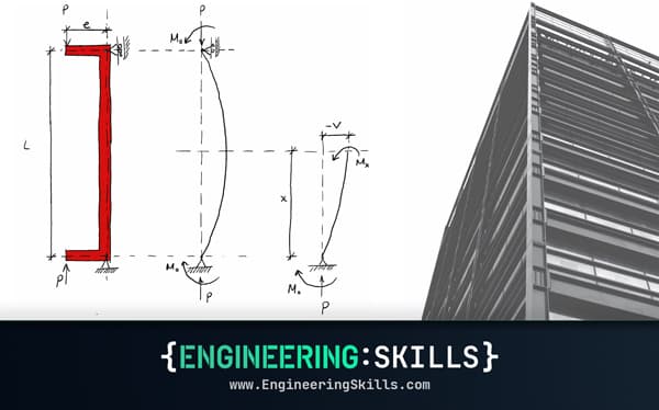
Column Buckling - Realistic Buckling Behaviour
Real-world columns rarely exhibit the strict mathematical buckling behaviour predicted for perfectly loaded, perfectly straight columns

Dr Seán Carroll
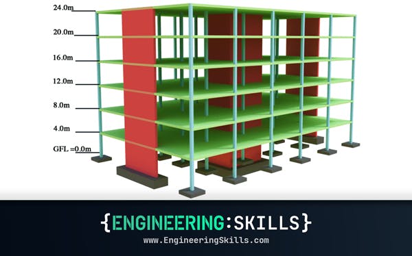
Structural Analysis and Stability – Symmetrical Structures
An introduction to common lateral stability structural schemes with numerical examples
Dr Seán Carroll