In this final lecture, we won't develop any new code - the hard work is done! The main aim of this lecture is simply to run another model through our code and see how it handles it. The Blender file and Jupyter Notebook are available, as usual, in the resources panel. You should consider this lecture as a prompt to go and build your own test models and get them converging in your new solver notebook.

The structure

The model we're going to analyse in this lecture is a simple cable-stayed lattice tower, Fig 1. These are very common structures, that you've no doubt come across at some point. The model will naturally include both bar and cable elements. We're not basing the model on any one structure, this model was simply borne out of some exploratory modelling in Blender - something I strongly encourage you to do following this lecture.

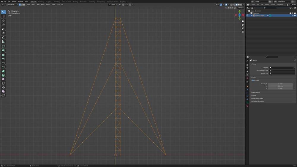
Fig 1. The Blender model of a cable-stayed lattice tower.

The tower is $30\:m$ high and $1\:m$ wide and is stabilised by 6 cables at third-points along its height. The four nodes at ground level will be modelled as pins and we’ll apply a lateral force along the right edge of the tower in the positive x-direction, Fig 2.

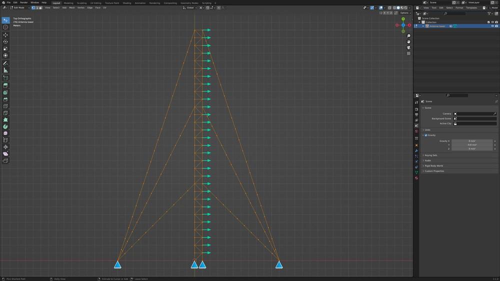
Fig 2. Support consitions and applied loading.

The modelling process uses basic vertex modelling operations in Blender. I won't document the process here, instead, you should watch the video to get a sense of how to build something similar. The data defining the structure is exported using the same scripts we wrote earlier in the course. The process of going from exploratory modelling to full simulation really is incredibly fast, once you familiarise yourself with the most basic Blender operations.

Simulation parameters

The simulation parameters are presented below. This is all we need to update in our solver notebook for any new simulation. The point load magnitude is set at $500\:N$ along the x-axis. Through trial and error, a combination of $5000$ force increments and a convergence threshold of $30\:N$ have been found to lead to a converging model.

#Constants
E = 70*10**9 #(N/m^2)
swt = True #Take self-weight into account 

areaCable = 0.00004 #(m^2) 
areaBar = 0.002 #(m^2)
gammaCable = 10 #(kg/m)10 Cable mass per unit length
gammaBar = 40 #(kg/m) Bar mass per unit length

preTension = 10 #Pre-tension applied to all cable elements
P = 500 #(N)🚨 Point load magnitude (and direction via sign)
pointLoadAxis = 'x' #🚨The GLOBAL axis along which point loads are applied

nForceIncrements = 5000 #Initial number of force increments for applied loading
convThreshold = 30 #(N) Threshold on maximum value of F_inequilibrium
itLimit = 10000 #The maximum number of iterations to achieve convergence
checkSlackAfter = 100

Simulation results

Running the simulation with these parameters leads to a final force imbalance of only $10\:N$, which gives us confidence in the final results. Figure 3 shows the deflected shape in force distribution within the structure. Qualitatively the behaviour is as expected considering the applied loading. We can see the self-weight of the cables causes them to sag, with the left to right deflection of the structure leading to larger sag on the right-side cables. The axial forces in the lattice tower are also reducing in magnitude as we move up the tower and the overturning moment generated by the lateral forces is reduced. So, from a qualitative perspective, the model output passes the sniff test.

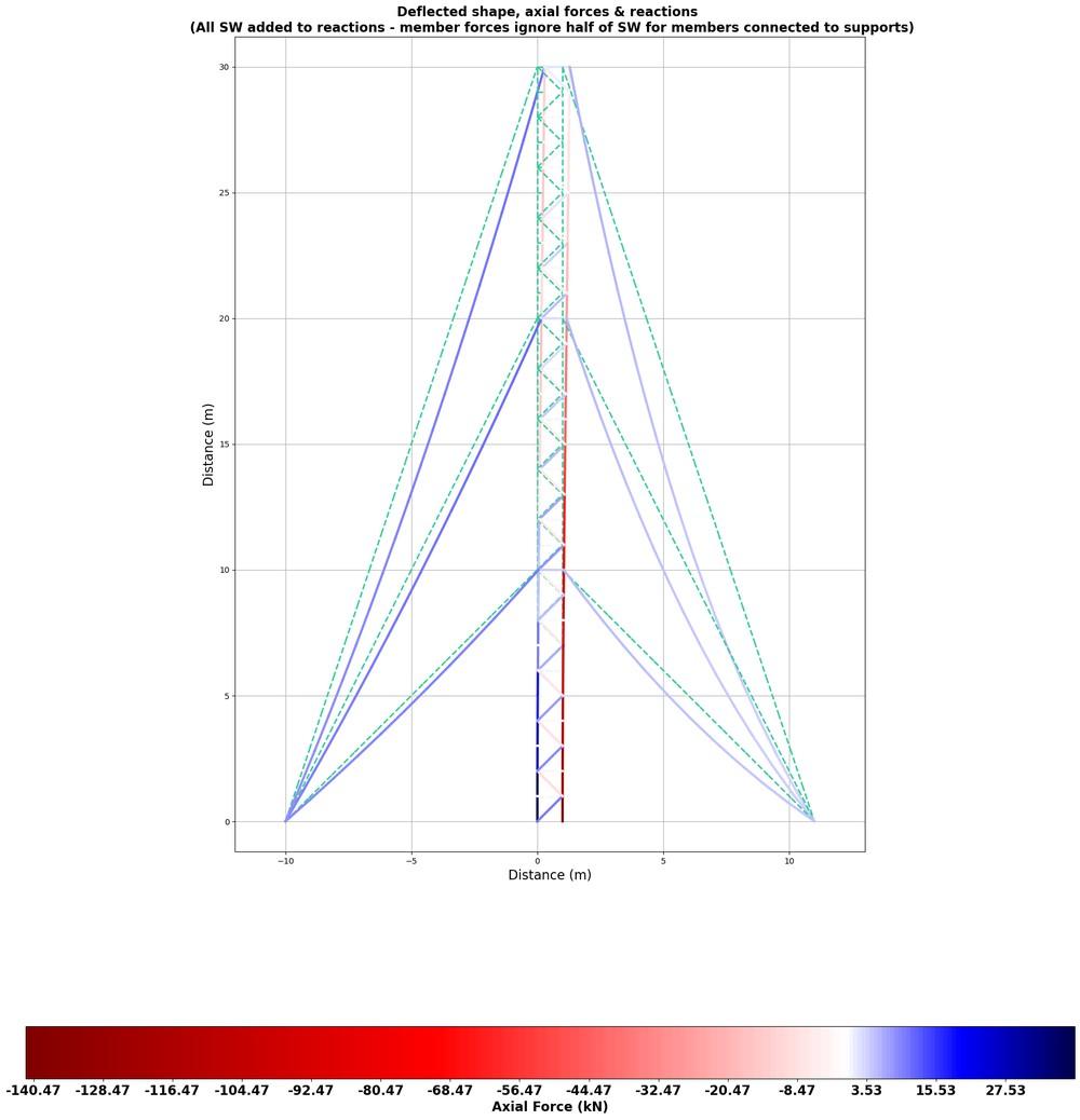
Fig 3. Deflected shape and axial force distribution.

If this analysis was part of a wider analysis and design exercise, the next task might be to alter the loading or structural properties or to assess the acceptability of these results against some design criterion. However, that's not something we'll pursue any further here. At this point, we're done!

Well done - you've built yourself quite a handy little toolbox.