In this lecture, we’ll write some code that allows us to solve Eqn. 1 numerically for
We'll do this by evaluating the equation repeatedly until we hit on a value of that satisfies the equation. Remember that for reference, you can download the complete Jupyter Notebook for this lecture from the resources panel above. The notes hereafter will assume that you're following along and writing code in your own Jupyter Notebook.
We start by importing some dependencies that make life a little easier for us.
# DEPENDENCIES
import math #Math functionality
import numpy as np #Numpy for working with arrays
import matplotlib.pyplot as plt #Plotting functionality
import csv #Export data to csv file
Next, we can define the parameters we specified at the end of the previous lecture.
#Input parameters
L = 10 #(m) Plan length
y_max = 2 #(m) Mid-span sag
sw = 981 #(N) Self-weight per meter of cable
Solve for the value of to achieve the desired sag.
Now we can plot Eqn. 1 for a range of different values of . I've specified values between 5000 and 10000 in steps of 0.1. Note that by rearranging the equation to equal zero, I'm plotting a homogeneous version of the equation. Therefore, we can identify the value of that satisfies the equation from the plot where the line crosses zero.
x = L/2 #(m) Location of target y_max
H=np.arange(5000,10000,0.1) #(N) #Range of H values to test

#Rearrange equation for y_max to be homogeneous (=0)
eqn=-y_max-(H/sw)*(np.cosh((-sw/H)*(x-(L/2)))-np.cosh((sw*L)/(2*H)))

fig = plt.figure()
axes = fig.add_axes([0.1,0.1,2,1])
axes.plot(H,eqn,'-')
axes.set_xlim([H[0], H[-1]])
axes.set_xlabel('H')
axes.set_ylabel('Eqn')
axes.set_title('Graphical solution')
axes.grid()
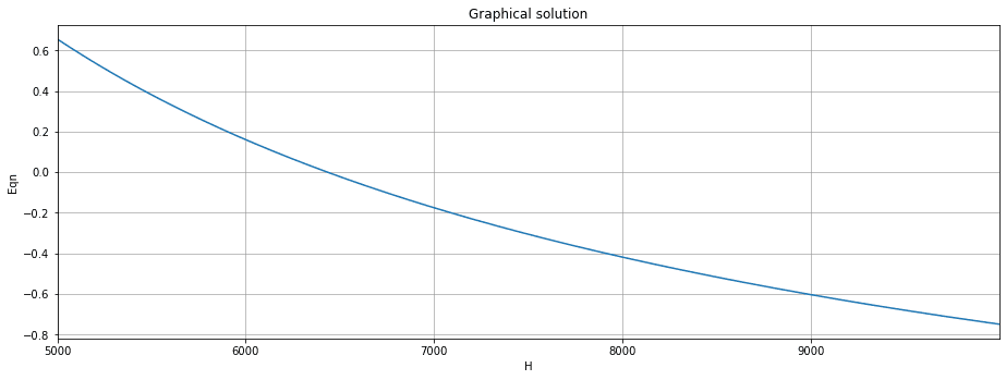
Fig 1. Plot of homogeneous catenary equation versus horizontal component of tensile force, .
We can see that the value of is something close to . To identify the specific value, we can loop through all of the values of eqn calculated above and test to see at what value of , eqn changes from being positive to negative. In doing so, it must have passed through zero.
Identify the specific value of
Although we can see graphically that the value of eqn does indeed change from positive to negative in this case, we'll write our code to take into account the potential for eqn to change from negative to positive should this arise for a different set of boundary conditions.
#Cycle through solutions and find value of H that satisfies the equation
for i in np.arange(0,len(eqn)-1):
  if eqn[i]<0 and eqn[i+1]>0:
    print(f'The required value of H is: {round(H[i],3)} N')
    H=H[i]
  elif eqn[i]>0 and eqn[i+1]<0:
    print(f'The required value of H is: {round(H[i],3)} N')
    H=H[i]
This code block outputs the following statement:
- The required value of is:
Plotting the catenary
We can see that after looping through all values of eqn, it changes sign when . As such, this is the value of that would develop for the specific
problem parameters specified above. Now that we know , we can use Eqn. 1 to plot the catenary. We'll break the span into linear segments, but you can break it into as many segments as you like.
n=12 #Break span into n segments (on plan)
delX = L/n #Segment length (on plan)

#Coordinates
x=np.arange(0,L+delX,delX)
y=-(H/sw)*(np.cosh((-sw/H)*(x-(L/2)))-np.cosh((sw*L)/(2*H)))

#Plotting
fig = plt.figure()
axes = fig.add_axes([0.1,0.1,2,1])
fig.gca().set_aspect('equal', adjustable='box')
axes.plot(x,-y,'-*')
axes.set_xlim([0, L])
axes.set_xlabel('x (m)')
axes.set_ylabel('y (m)')
axes.set_title('Catenary')
axes.grid()
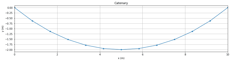
Fig 2. Twelve segment catenary
Calculate the catenary length
Next, we'll calculate the maximum value of the cable tension force (at the supports). To do this, we need to know the vertical component of the tension force. We already know the self-weight per unit curved length of cable, so now all we need to determine is the curved length.
We'll approximate this by calculating the length of the segments we've used to approximate the catenary. Obviously, your approximation would be improved by increasing the number of segments. We'll cycle through each segment, calculate its length and add it to a running total of all segment lengths.
L_cat=0 #Initialise the length

#Cycle through each segments and determine the length
for i in np.arange(0,len(x)-1):
    dx = abs(x[i+1]-x[i])
    dy = abs(y[i+1]-y[i])
    L_cat += math.sqrt(dx**2 + dy**2)

print(f'The cable length is approximately {round(L_cat,3)} m')
- The cable length is approximately
Calculate the max tension at supports
Now we can calculate the total self-weight and divide it by to calculate the vertical component of the cable tension force at supports, . We can determine the resultant of and to determine the maximum cable tension, .
V = 0.5*(L_cat*sw) #(N) Vertical reaction at support
T_max = math.sqrt(H**2+V**2) #(N) Cable tension at the support

print(f'The vertical reaction is {round(V,2)} N')
print(f'The maximum cable tension at supports is {round(T_max,2)} N')
- The vertical reaction is
- The maximum cable tension at supports is
Export catenary coordinates and segment definitions
Finally, we'll export the coordinates of the vertices or nodes of the catenary and the definitions of the segments or edges that make up the catenary. The segment definitions are simply the node numbers at each end of the segment. We'll use these a little later in the course.
The export code here is standard export boilerplate code. We're exporting the nodes and segments to two comma-separated value (csv) files names Vertices.csv and Edges.csv located on the desktop. Make sure to change the file path to reflect your computer (unless you also happen to be called Sean, of course!)
#Initialise containers
vertices = np.empty((0,2),int) #Nodal coordinates
edges = np.empty((0,2),int) #Segment definitions

#Cycle through nodes and determine coordinates and member definitions
for i in np.arange(0,len(x)):
  vertex = np.array([x[i], -y[i]])
  vertices = np.append(vertices, [vertex], axis=0)

  if(i<len(x)-1):
    edge = np.array([i+1, i+2])
    edges = np.append(edges, [edge], axis=0)

#Export vertex coordinates to CSV file
filename = "/Users/Sean/Desktop/Vertices.csv" #UPDATE PATH
# writing to csv file
with open(filename, 'w') as csvfile:
  csvwriter = csv.writer(csvfile)  # creating a csv writer object
  csvwriter.writerows(vertices) # writing the data rows

#Export edge/element definitions to CSV file
filename = "/Users/Sean/Desktop/Edges.csv" #UPDATE PATH
# writing to csv file
with open(filename, 'w') as csvfile:
  csvwriter = csv.writer(csvfile)  # creating a csv writer object
  csvwriter.writerows(edges) # writing the data rows
This completes our study of linear cable behaviour. Over the last 4 lectures, we've seen how to derive and model linear cable behaviour. This linear model will later serve as a baseline to compare our non-linear solver behaviour against.
If there is one key takeaway message here, it's that all of this modelling is only valid if the cable’s geometry does not change under load. Once this assumption is not met, the behaviour becomes non-linear. This is what we'll start to explore in the next section.
Please log in or enroll to continue
If you've already enrolled, please log in to continue.
Non-linear Finite Element Analysis of 2D Catenary & Cable Structures using Python
Build an iterative solution toolbox to analyse structures that exhibit geometric non-linearity due to large deflections.
After completing this course...
- You will understand the concept of geometric non-linearity and when it should be considered.
- You will understand how to modify the axially loaded element stiffness matrix to account for large deflections and changes in geometry.
- You will have implemented a Newton-Raphson iterative solution algorithm that seeks to converge on the deformed state of the structure.
- You will have a workflow that leverages open-source modelling tools in Blender to quickly generate the initial structural geometry.