Using Gmsh to generate finite element meshes for floor structures in Python

Welcome back to our series on modal analysis of floor slabs using OpenSeesPy and Gmsh. In part 1, we worked on using OpenSeesPy to build a finite element model and perform a modal analysis. If you missed that, read part one here…Calculating floor slab vibration modes using OpenSeesPy. Here, in part 2, we’re going to focus on mesh generation using the Gmsh Python API. In part 3, we’ll bring it all together to build a complete meshing and modal analysis toolbox!

1.0 Supercharging our modal analysis pipeline

You’ll recall that in part 1, the main objective was building and validating our modal analysis code. To do this, we manually generated a simple finite element mesh consisting of rectangular elements (since the case-study plate/slab was a simple rectangle).

For practical analyses, our approach to mesh generation in part one can only take us so far! There are two main steps to any finite element analysis: mesh generation and system solution, i.e. solving the system of simultaneous equations that describe the structure. OpenSeesPy handled the system solution for us. Now, Gmsh will handle the (not insignificant) task of mesh generation.

We briefly introduced Gmsh in part 1 - it’s a powerful finite element mesh generator that can be used to generate finite element meshes for 2D and 3D structures. We’ll focus here on generating 2D meshes, but this really only scratches the surface of what this extensive library is capable of. It’s worth poking around the Gmsh website to get a sense of just how impressive this open-source tool is. You can get a really good sense of the overall structure of the library in the Overview of Gmsh section of the documentation.

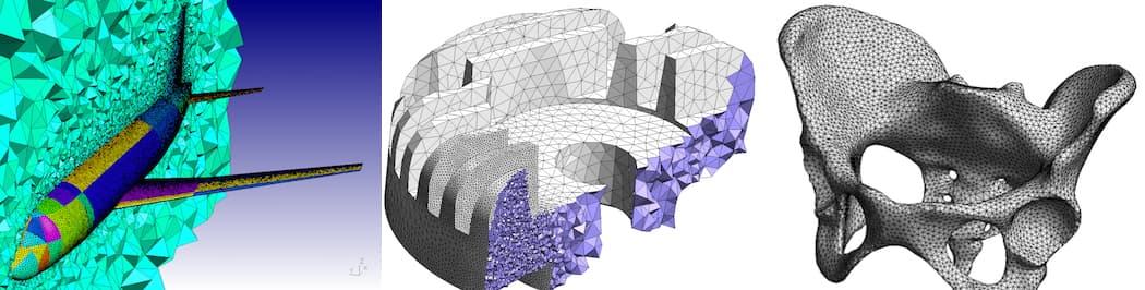
Images of various mesh generation outputs using Gmsh | EngineeringSkills.com

Fig 1. Images of various mesh generation outputs using Gmsh [from the Gmsh website].

GUI versus API

Gmsh can be used through a graphical user interface (GUI) or via one of its various application programming interfaces (APIs) - it has APIs for C++, C, Python, Julia and Fortran.

Since we’re building a scripting-based analysis pipeline in Python, we’ll use the Python API, but I would encourage you to take a look at the GUI too - particularly if you’re getting into 3D structures where visualisation with matplotlib starts to get cumbersome.

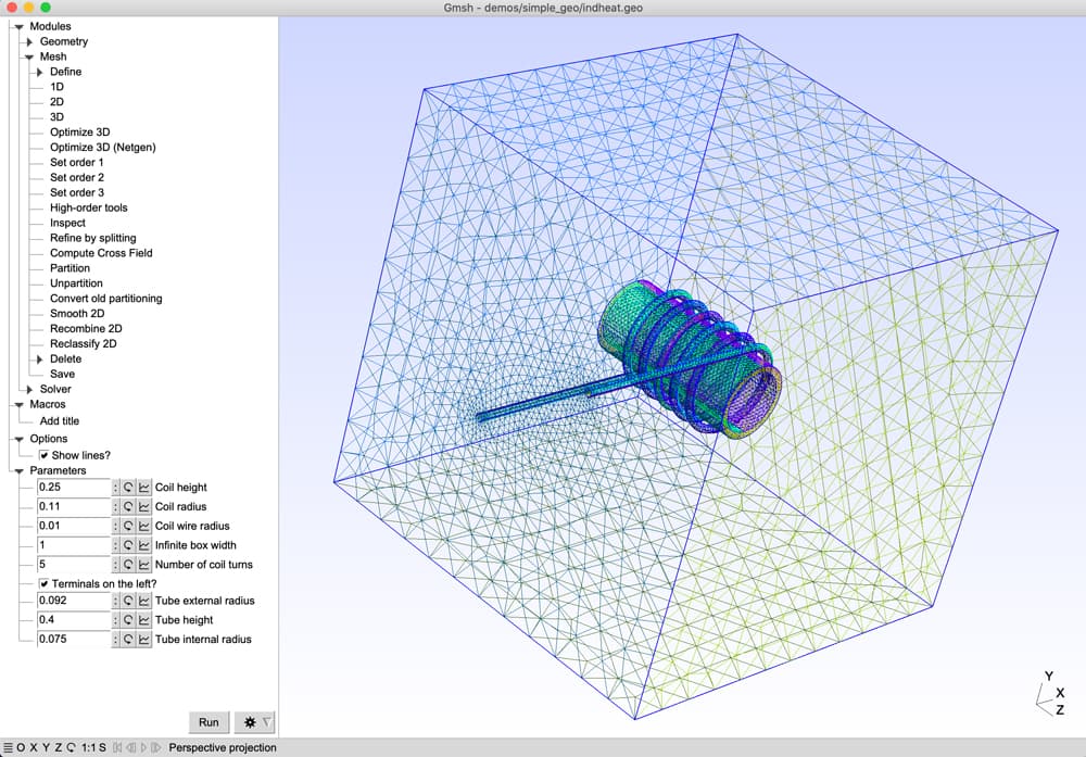
Fig 2. The Gmsh GUI [from the Gmsh website].

Gmsh has very extensive and mature documentation. Probably the most helpful section for getting to grips with the library is the series of tutorials that progressively introduce Gmsh capabilities. The Python-specific versions of these tutorials can be found here.

One final note I should add relates to Gmsh's license. Gmsh is distributed under the terms of the GNU General Public License (GPL). From the Gmsh website...

In short, this means that everyone is free to use Gmsh and to redistribute it on a free basis.

The license is quite permissive but you should read through the terms of the license to make sure it's compatible with your intended use of the API.

Remember that the aim of this EngineeringSkills series is to help you use freely available open-source libraries (OpenSeesPy and Gmsh in this case) to perform quite complex numerical analysis. These analyses are typically gated behind commercial software packages with very hefty price tags!

Will we recreate the full feature set of a large commercial analysis package? Clearly not, but in many cases, you don’t need the full feature set to accomplish the task on your desk today!

Ultimately, my hope is that this series, like all of our Python library tutorials, gives you a sense of what’s possible with the amazing tools we have at our fingertips…thanks to the hard work of so many researchers and open-source developers!

Tutorial breakdown

📍 2.0 Rectangular QUAD mesh generation

In the next section, we’re going to dive right into mesh generation with Gmsh. By the time you’ve worked through this tutorial, you’ll have built quite a sophisticated mesh generation tool. But we’re going to build it incrementally so it never gets too overwhelming!

Our first step is to generate a mesh for a simple rectangular slab. This will introduce us to about 90% of the Gmsh code we’ll need to write. When this first iteration of our meshing function is complete, we’ll improve it, bit by bit, as we continue through the tutorial.

📍 3.0 Visualising the finite element mesh

In section 3, we’ll write some code that takes the mesh data we generated in step two and plots it using matplotlib. This will allow us to actually see the finite element meshes we’re generating. Our approach here will again be to build the basic plotting function and then incrementally improve it.

📍 4.0 Polygon QUAD mesh generation

With the foundations of a meshing and plotting function built, we make our first incremental improvement by generalising our meshing function to work on general polygons that don’t have 4 sides - we can refer to these as n-gons.

📍 5.0 Implementing slab openings (mesh holes)

As we’re building a tool to apply to floor slabs, we’re going to need to accommodate holes in the slab! So, our next improvement will be to pass in data defining slab openings and have our mesh generator respect these voids in the slab.

📍 6.0 Adding known nodal points (for point/column supports)

In section six, we implement our final enhancement and further generalise our meshing function to allow the definition of discrete mesh points. This will allow us to specify locations in our slab mesh were we specifically want nodes to be positioned. This will be important later when it comes to adding vertical restraint provided by columns at pre-defined locations.

📍 7.0 Wrapping up and what’s next?

Finally, in section seven, we’ll comment briefly on progress so far, mention some additional features you might like to implement and tee up part 3 in the series, where we combine our new meshing functionality with the modal analysis work we did in part 1.