Finite Element Analysis and Structural Behaviour Modelling Case Study

1.0 Introduction and Objective

To perform structural analysis, particularly for complex structures, we need to bring a lot of skills to the table. We need a sound understanding of structural mechanics, an appreciation for how our modelling assumptions relate to real-world or ‘as-built’ behaviour, some intuition for global structural behaviour and a healthy dose of skepticism about the validity of our analysis. A good approach is to assume you’ve done something wrong until you’ve exhausted all opportunities to prove otherwise. Very often, the most practical way forward is to build a high fidelity computer model and perform a finite element analysis – but this should rarely be the starting point.

This post is part tutorial, part opinion piece on the role of computerised (finite element) structural analysis and part hat-tip to a fantastic structure, the Tintagel Footbridge, located an hour down the road from me in beautiful Cornwall, England. The aim of this post is ultimately to use the Tintagel footbridge as a case study to explore structural behaviour and show how we can build up an understanding of the structure through analysis of increasingly complex models. Throughout this post we’ll make use of finite element analysis codes developed in various DegreeTutors courses. You can access the codes and learn how to build them for yourself by following the links provided.

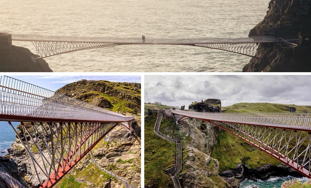
The Tintagel Footbridge, Cornwall, England. Completed in 2019

In this post I’ll make repeated reference to the finite element method and finite element modelling. In broad terms what we’re really talking about is matrix methods of structural analysis, wherein the structure is divided into finite elements connected at nodes. The stiffness matrices that relate forces with displacements for each element are combined cleverly into one big stiffness matrix for the whole structure. Knowing the forces applied at nodes, we can invert this structure stiffness matrix and determine displacements at each node, et voila – the structure is ‘solved’! I’ve written a first principles tutorial here. This is the fundamental idea behind finite element analysis. Things get more interesting when we start to think about different types of elements; bars, beams, 2D solids, shells etc. But we’re going to focus on axially loaded bar elements and beam elements exclusively here.

1.2 The Finite Element Analysis Trap

I’ve had the good fortune to work with thousands of engineering students over the years. I never cease to be amazed by their creativity, curiosity and willingness to roll up their sleeves and get stuck into whatever challenge they face. Their enthusiasm is often accompanied by a natural and understandable dose of naivety for structural behaviour and how to tease apart how a structure works. This is to be expected, after all structural analysis is one of the hardest skills to develop as an undergraduate or even graduate engineer. As a result, students quite often come unstuck when they jump prematurely into computer modelling of structural behaviour.

With such easy access to incredibly powerful software the temptation to bypass preliminary hand analysis techniques or exploratory modelling can be great. What student would honestly prefer to crunch through pages of hand calculations (then start again when you realise you made a mistake on page one!) when a much more attractive and speedy 3D model can be built? A computer model gives instant gratification, deflected shape animations, stress distributions, bending moment diagrams and all with the subtle suggestion that the output must be correct. This is a trap all engineers, myself included, have stumbled into at some point in their education and/or career!

However we need to remember, our finite element model us just that, a model that approximates the behaviour of the actual structure. It’s only as good as the assumptions used to build it. There is ample room for error to creep in when we try to map our structure from the real-world into a 3D model. I claim no special expertise here – for me, deciding how to approximate various features of a structure within a finite element model is often a huge challenge. After that the mechanics are all relatively straight-forward, but it can all be for nothing if the inputs are wrong.

1.3 Finite Element Analysis + Iteration = Confidence

So, should we throw off finite element modelling and all revert back to Brunel’s day and analyse everything by hand? Just the suggestion is enough to bring on a cold sweat and make me consider a career in architecture! Modern engineering consultancy would not be financially viable without the efficiencies offered by computerised analysis and design – we need finite element analysis. So how do we link our understanding of fundamental structural behaviour with the output of complex computer models and have confidence in our predictions?

One way is to iterate our way through increasing levels of complexity, making sure we fundamentally understand the behaviours predicted at each iteration. This way we can scaffold our understanding by building up incrementally with models of increasing fidelity and detail, from simple models to full 3D finite element models. This allows us to tease out the structural behaviour and build a picture of how the structure works. It means we arrive at the final set of result with context and a history of how the preceding results lead us here. If we start (and finish) by building our most complex representation of the structure first – how can we judge the validity of our output? If that’s the only data we have, we have no context in which to consider our results.

In this post, we’ll apply this iterative approach to the Tintagel Footbridge by starting with the simplest representation possible and incrementally stair-stepping our way to a full blown 3D finite element model. I have no ‘insider information’ for this bridge, so we’ll be making some guesses and assumptions about dimensions and materials along the way. Our focus here is on demonstrating a general approach to modelling rather than trying to capture the exact behaviour of this structure – we just don’t have the necessary detail for that.

2.0 The Tintagel Footbridge: Our Case-Study Structure

The Tintagel footbridge is located on Cornwall’s north coast. It spans a rocky chasm that was left by the collapse of a natural land bridge between the mainland and a rocky outcrop of historical significance. According to English Heritage, the land bridge collapsed some time between the 14th and 17th century. You can read more about the bridge replacement project on the English Heritage website. Wikipedia also has a good article on the history of the site.

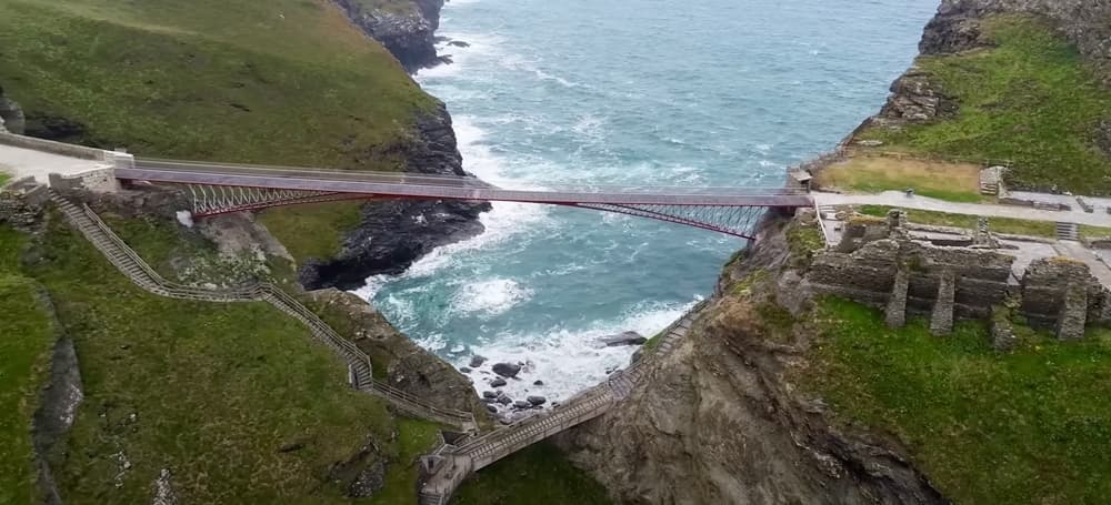
View of the old (lower) and new (upper) Tintagel footbridges

The new footbridge was completed in August 2019. This greatly improved access to the rock outcrop which previously could only be accessed by steep stairways on either side of a short timber footbridge. The Architects were William Matthews Associates and the Structural Engineers were Ney & Partners. The bridge spans 68.5 m and appears to combine a number of structural mechanisms which we’ll explore further below.

At the mid-span, there is a 40 mm gap in the deck. This has some symbolic significance in the context of the site and is a nice feature that adds a little drama for visitors crossing the bridge. There are many examples in the media of the bridge being described as two independent cantilevers. This is interesting, however there are two round steel bars that span across the gap. If considered as two separate bridges, a more accurate description may be propped cantilever or a pair of mutually propped cantilevers; although I can see the nuance being lost on a non-technical audience. Having said that, the connecting bars a very slim, it may well be that modelling each half of the bridge as a cantilever structure is reasonably accurate. For the purposes of structural modelling, we’re likely to model this connection at the mid-span as a rotational pin allowing transmission of shear and axial forces. Clearly bending won’t be transmitted through this joint.

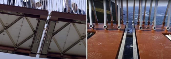
View of the steel pins spanning the 40mm gap at the centre of the bridge.

2.1 Loading, Geometry and Assumptions

As I mentioned above, we’re going to have to make a number of assumptions to facilitate our analysis. These mainly relate to dimensions, materials and loading, I’ll highlight these as we go. As a starting point, I’ve constructed a 3D model of the bridge that captures the essence of the structure. It’s not an exact replica – but close enough. We’ll use this as a proxy for the structure and from this point forward, we’ll base our analysis on this 3D model (you can explore the model in detail below). If you have 2D plans for your structure, that would work fine too. I’m estimating a deck width of approximately 2.3m, with the distance between main longitudinal members being approximately 2.55m centre to centre.

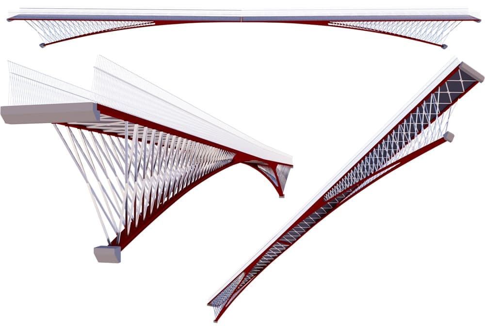
Renderings of the 3D bridge model on which are analysis will be based.

Section sizes & properties We’re going to have two types of element in our models, beam elements that transmit axial forces, shear forces and bending moments and bar elements that resist axial loads only. All bar elements will be square hollow sections with cross-section dimensions 80mm x 80mm and a 6mm wall thickness. You can see below which elements are being modelled as beams and bars.

Structural members modelled as Beam and Bar elements in our finite element model.

For the beam elements I’ve estimated a doubly-symmetrical box girder with cross-section dimensions detailed below. In the actual bridge where the inclined member joins the horizontal deck beams, the section size increases locally as the members merge. This is slightly exaggerated in the 3D model. In our modelling we’re initially going to ignore this section change and simply assume that the horizontal and inclined members meet at a node.

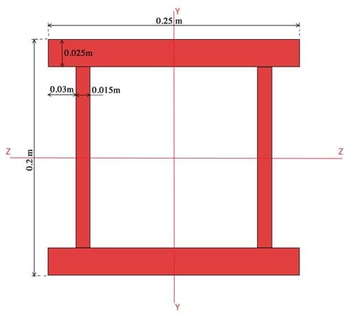
Beam element cross-section

The area of the cross-section is,

Using the parallel axis theorem, we can determine the second moment of area about the centroidal $Z$ and $Y$ axes. Considering the major $Z$ axis first,

Next the minor $Y$ axis,

Loading
We’ll scheme up some loads to work with next. Remember, the objective here is to get something approximate to work with so we’re not too bothered about a detailed or code-compliant load takedown for this exercise. Based on information available on the English Heritage website, I’m assuming a deck buildup of:

• $10\:mm$ steel plate $[0.77 \:kN/m^2]$
• $30\:mm$ bed of sand $[0.57\: kN/m^2]$
• $60\:mm$ slate (on end) walking surface $[1.68\: kN/m^2]$

This gives an imposed ‘dead’ or permanent load of $3.02$, say $3\: kN/m^2$. If we assume a deck width of $2.3 m$. this would yield a uniformly distributed load (UDL) of $3.45\: kN/m$ along each longitudinal main beam. If we assume an imposed or variable load of $5 \:kN/m^2$, this would give us a UDL of $5.75 \:kN/m$ along the main beams. The self-weight of the structural elements will be calculated within our Python code based on the cross-section and material properties provided. So we have a service limit state (SLS) load, (excluding self-weight) $9.2 \:kN/m$ and an ultimate limit state (ULS) load (again excluding self-weigh) of about $15 kN/m$.

3.0 Preliminary 2D Finite Element Modelling

Now we’re finally ready to start some structural modelling and analysis. We’ll start with a simple model  that doesn’t even warrant finite element analysis and work our way up to something that reasonably approximates our structure in 2 dimensions. Then we’ll expand into a 3D model in the next section. For the analysis in this section we’ll apply half of our ULS loading of $15 kN/m$ as we’re essentially modelling half of the structure and we’ll ignore self-weight. For our 2D analysis we’re more interested in the relative behaviour of our models. For the analysis in this section we’re going to use the solver code developed in the course ‘Beam & Frame Analysis using the Direct Stiffness Method in Python‘.

3.1 Step 1: Fixed-fixed beam

One of the simplest ways we might imagine spanning this gap is with a simple beam. Clearly this is not a practical solution, but from a modelling stand-point it makes sense to start with a model we’re comfortable with and build from there. We’ll start by assuming fixed supports. For this model, we can obtain the support and span moments directly from reference tables. Similarly the mid-span deflection is easily obtained.

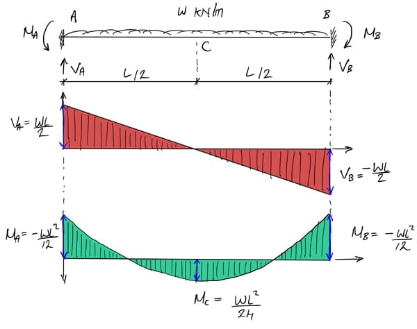
Simple fixed-fixed beam model with shear force diagram (red) and bending moment diagram (green)

The maximum magnitude shear at supports is obtained as,

We can evaluate the support moment magnitudes to be,

The span moment is observed to be half the magnitude of the support moments, $M_C = 5865.3/2 = 2932.7\:kNm$. For completeness we’ll calculate the mid-span deflection, $\delta_C$ noting that $E = 200\:kN/mm^2$ and $I = 104.79\times10^6\:mm^4$.

At the risk of stating labouring an obvious point, this is obviously not a viable structure, the beam will yield and fail long before these actions are ever actually experienced. The calculations here simply serve as a convenient starting point for our analysis. For this simple model we certainly don’t need to build a finite element model, however for completeness and consistency we’ll solve this structure using the exact same techniques and solver code we’ll use throughout this section. This gives us a good foundation as we’re starting with a simple structural model that we fully understand and can directly link between our hand-analysis and computer output.

Our beam is constructed using beam elements, each with six degrees of freedom spanning between 43 equally spaced nodes. The UDL has been applied through a process of evaluating equivalent nodal actions. The solver output is summarised below.

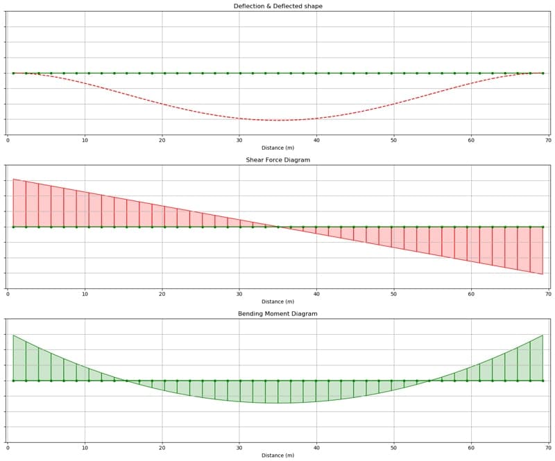
Qualitative deflected shape (top) shear force diagram (middle) and bending moment diagram (bottom) for the fixed-fixed beam model.

Closer inspection of the solver output below reveals full agreement with our hand calculations. No great surprises here.

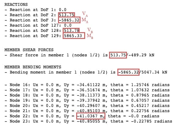
Extract of solver text output confirming agreement with values obtained in hand calculations

3.2 Step 2: Fixed-fixed beam + pin

The next complexity we can add is the mid-span rotational pin. To facilitate this within our finite element code, we’ve derived an element stiffness matrix with a rotational release at node i (for the element to the right of the pin) and another element stiffness matrix with a rotational release at node j (for the element to the left of the pin).

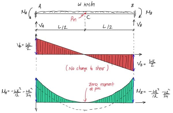
Simple fixed-fixed beam with mid-span pin model with shear force diagram (red) and bending moment diagram (green)

Again this is quite a straightforward structural model and we can quite easily deduce the influence of the pin on the bending moment diagram; i.e. reducing the mid-span moment to zero and essentially transferring this moment onto the support moments. Obviously there is no change to the shear force diagram and the pin serves to increase the mid-span deflection and alter the deflected shape. Again we can confirm our deductions with the output from our finite element model. Worth noting that introduction of a mid-span pin has increased the mid-span deflection to $\delta_C = 123.2\:m$!

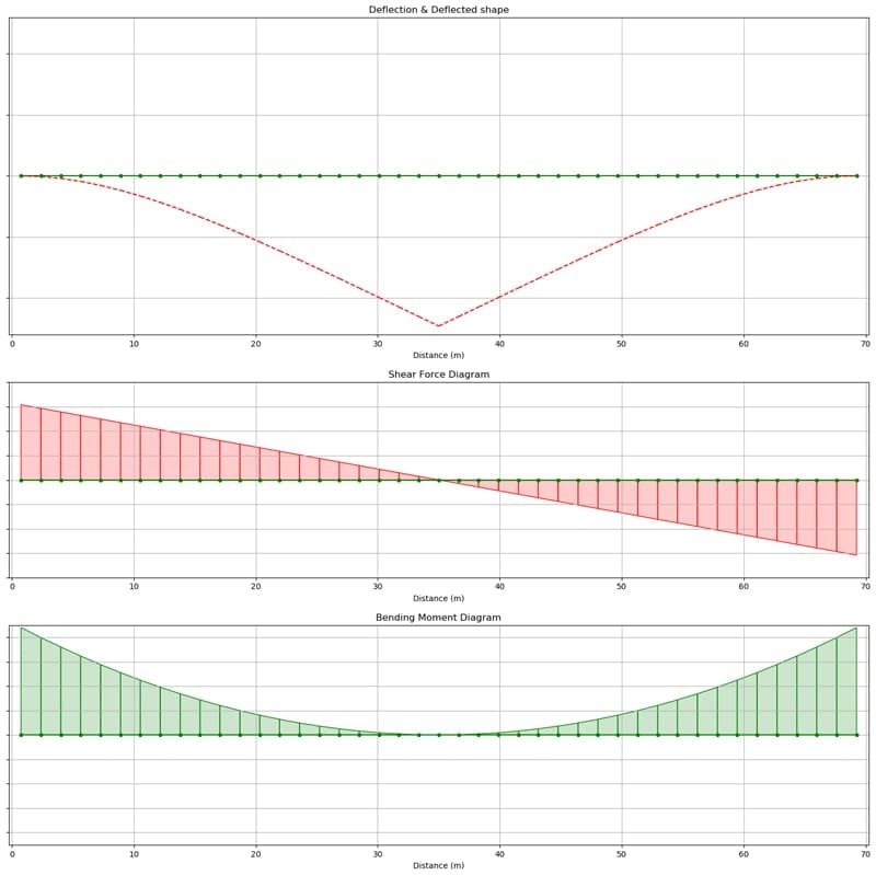
Qualitative deflected shape (top) shear force diagram (middle) and bending moment diagram (bottom) for the fixed-fixed beam with mid-span pin model.

3.3 Step 3: Simply-supported propped beam with pin

The beams in step’s one and two are not realistic solutions, they serve mainly as a modelling exercise to give us a foothold from which to progress our analysis. In this step we’ll start to move towards a more credible structure and introduce inclined propping supports to our beam. We’ll also move away from fully fixed supports and now model our supports as pins.

The inclined props will be modelled as straight axially loaded elements for now. This will cause our main beam to behave as a continuous beam with sinking supports. So although we’re not going to directly compare quantitative hand analysis with our model output, we can think about what the qualitative behaviour should be and confirm that this accords with our solver output. Remember, the goal with this preliminary modelling is to work our ways towards a complex model by understanding the layers of complexity along the way.

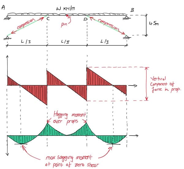
Simply supported propped beam with pin model with shear force diagram (red) and bending moment diagram (green)

We expect our inclined props to go into compression. The vertical component of the compression force in the props will introduce a step change in our linear shear force diagram. Our bending moment diagram should show hogging moments developing over the props. We can use the locations of zero shear to identify where the local maximum sagging moments will occur in the spans. 

Below we can see the finite element model from step 2 altered to include two inclines axially loaded props (shown in green).

Comparison between target structure (top) and simplified finite element model (bottom). Blue elements are beam elements, green elements are axially loaded bar elements.

Examining the solver output below; the top diagram is an axial force diagram with compressions members indicated in red and tension members indicated in blue. As expected the props are in compression, with the central span also experiencing compression. Also as expected, we have hogging moments developing in the beam over the prop supports. Recall that these axially loaded props are modelled as 80x80x6 square hollow sections, so in reality they will have buckling considering the axial load transmitted into them and their unrestrained length. Nevertheless we now have a sense of what inclined props will do for the overall behaviour of the structure – critically they will reduce the magnitude of the moments developed in the main beam.

Props (if they didn’t buckle) also serve to dramatically reduce the mid-span deflection down to $\delta_C = 2.6\:m$ (note that the scale of the deflected shape plots is not consistent between modelling steps).

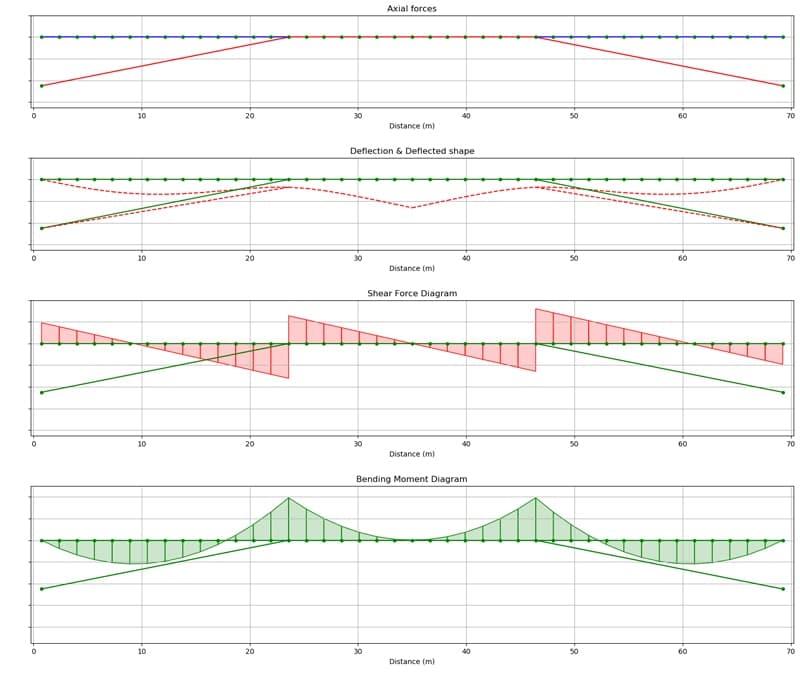
Axial force diagram (top) with red elements in compression and blue in tension, qualitative deflected shape (second from top) shear force diagram (second from bottom) and bending moment diagram (bottom) for simply supported propped beam with pin.

3.4 Step 4: Simply supported beam + arched props

In this step, we’ll better approximate the nature of the inclined props my modelling them as beam elements. We’ll generate the arching shape by gradually rotating each linear beam element to produce a ‘faceted’ beam. The arching inclined support is more in keeping with the actual structure. We’re also altering the location of the arch supports to better reflect the geometry of the actual structure. The lower two supports will now be modelled as fixed or built-in supports.

We can see that the arching geometry of the inclined members means they actually provide less effective support to the main beam. They join the main beam at quite a flat trajectory, which effectively increases the central span of the main beam (by comparison to the step 3 model). We can see this by noting the increased magnitude hogging moment $(1282\:kNm$ versus $981\:kNm)$ and significantly larger mid-span deflection, $\delta_C = 5.3\:m$.

Now that we’re modelling the props as beam elements, we expect to see moment and shear generated in these elements and sure enough that’s what we see. Note that the fact that the arch supports are made up of linear segments (faceted)  we set step changes in the shear force diagram that approximate a linear variation in shear while the bending moment diagram approximates a polynomial curve. This is due to the discrete nature of our model. The more elements used to approximate the curve the smaller this ‘stepping effect’ becomes as the change in angle between adjacent finite elements reduces.

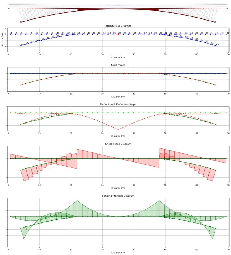
Elevation of the structure (top), simplified finite element model (second from top), axial force diagram (third from top) with red elements in compression and blue in tension, qualitative deflected shape (fourth from top) shear force diagram (second from bottom) and bending moment diagram (bottom) for simply supported beam with arched props.

Clearly the changes we’ve made in this modelling step have led to a deterioration of the structural performance, even if they do better reflect the geometry of the real bridge. But we’re still missing one big component of the real structure – those axially loaded truss style elements.

3.5 Step 5: Truss + Arch + Beam

Now we’re going to approximate the truss behaviour of the real structure by implementing axially loaded propping elements within our 2D model between the main beam and arching support. We expect this to significantly reduce the bending moments within the structure and also the mid-span deflection. Although these new elements won’t do much to address deflection that occurs in the central portion of the structure. Our simplified 2D model is shown below. The truss elements are arranged in a criss-cross pattern and members are not connected at their point of intersection.

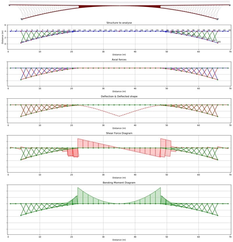
Elevation of the structure (top), simplified finite element model (second from top), axial force diagram (third from top) with red elements in compression and blue in tension, qualitative deflected shape (fourth from top) shear force diagram (second from bottom) and bending moment diagram (bottom) for simply supported beam with arched props.

We can see that the two outer quarters are clearly behaving as cantilever trusses and have been significantly stiffened by the internal propping/bracing elements. The axial forces in these props are alternating between tension and compression as we might expect for this cross-bracing pattern. Deflections and bending moments in these outer quarters have been drastically reduced. We can see that the large mid-span deflection is due to the long and slender central span. This won’t be helped by the presence of the rotational pin at the mid-span point but it has been reduced back down to $\delta_C = 3.6\:m$, not as low as we saw in step 3 $(\delta_C = 2.6\:m)$ but better than step 4 ($\delta_C = 5.3\:m$).

When we compare our simplified 2D model to our 3D architectural model, we can see that our simplified model exaggerates the flexibility of the central span. In reality, the central portion of the bridge is not as slender as our 2D model suggests. However this is still a useful exercise to establishing the influence of different structural elements on the global behaviour of the structure.

We’ve observed that the bridge likely benefits from a number of different structural mechanisms. Most prominently, truss behaviour as demonstrated by the modelling in this step. We also have cantilever or propped cantilever bending in the central span of the beam. Presently this is accounting for the great majority of the deflection in our simplified model. The trusses themselves are also cantilevering from their supports of course. We also have arching action at play as we notice the inclined props and central span are all in compression.

At this point we’ve learned about as much about the qualitative structural behaviour as we can from simplified 2D models. We could further refine these 2D models and perhaps get a better approximation of the quantitative behaviour. But instead, we’re going to try and refine our models in 3D to get a more complete picture of the behaviour.

Again, it’s worth emphasising that we’re jumping to 3D having established a feel for how the structure behaves in 2D. This means that if we see something in our 3D model output that doesn’t look ‘right’ we’ll have the reference point of our 2D models to compare against, qualitatively at least. With enough practice and experience, you may be able to form a good idea of how the structure should behave and as such you can bypass 2D exploratory modelling. But if you’re unfamiliar with finite element modelling and computer based analysis in general, or you’re dealing with a complex structure – simplified iterative analysis as we’ve done here is a good idea.

4.0 3D Finite Element Modelling

In this section we’ll discuss the analysis of a 3D finite element model of our structure. We’re going to look at 2 versions of the finite element model, then we’ll consider a pure cantilever version of the bridge (i.e. two independent cantilever trusses that ignore the pin connection in the middle). For brevity, we’ll confine our discussion to a comparison of mid-span deflections and overall deformed shape of the different models.  All of the modelling, analysis techniques and codes used in this section are developed and discussed in the course, ‘Finite Element Analysis of 3D Structures using Python’.

4.1 3D Finite Element Analysis – Model 1

The 3D structural model is based on the geometry of the architectural model. The same approach to element selection has been used as in our 2D modelling; cross-bracing in the deck and truss elements have all been modelled using bar elements that resist axial load only. With all other elements being modelled as beam elements resisting axial force, shear force and bending moment. Our $15 \:kN/m$ uniformly distributed load is now been applied to both longitudinal deck beams. All other material properties and cross-sectional dimensions are the same as in our 2D models.

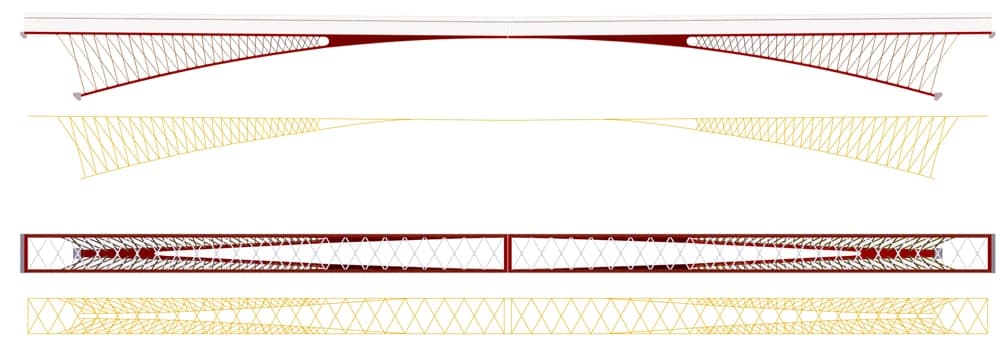
Elevation and plan of the bridge showing a comparison between the architectural (upper) and structural (lower) models.

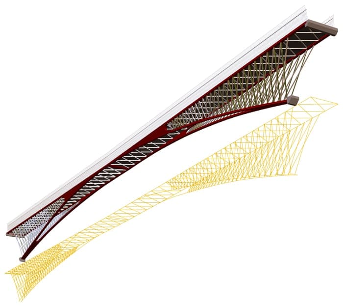
3D view of the architectural and structural bridge models.

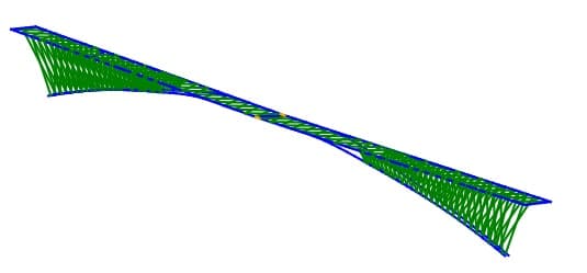
Structural model with axially loaded bar elements shown in green and beam elements shown in blue. Pinned beam elements are shown in yellow at the mid-span location.

Note from the model visualisations above that the central span of the structural model is again very slender when compared to the architectural model. Remember that the beam elements have the cross-section described in section 2.1 above and have an overall depth of only $200\:mm$. Based on what we know from our 2D modelling, we expect this to lead to large mid-span deflections despite the outer truss portions of the structure remaining relatively rigid with comparatively little deflection. 

The image below shows the deflected shape of the structure overlayed on top of the original structural model. Note that these deflections are shown at the same scale as the structure, i.e. they are not scaled up. As we might imagine, as the depth of the cantilever truss reduces towards the mid-span, the vertical deflection increases. However the slender central span experiences the largest deflections in agreement with our rudimentary 2D model. The mid-span vertical deflection is $1.3\:m$ (down from $3.6\:m$ in 2D modelling step 5).

Deflected shape of version 1 of the 3D finite element model. Deflections shown at same scale as the structure.

Something that only becomes apparent when we consider the 3D model is the ‘out of plane’ or ‘into the page’ deformation of the structure. We can see from the deformed shape below that the out of plane stiffness of the arched legs is is far too low and we observe large lateral deflections of these legs to the point that they cross over each other! This is likely due to the fact that we haven’t accurately modelled the geometry of the structure in this region, we’ve modelling each arch leg individually connecting into a support. In reality, we can see from the architectural model that these arch legs actually combine onto a single wider leg as they approach their supports. This will greatly increase the out of plane stiffness of the arching structure. This is a good example of structural behaviour that we can only fully appreciate with a 3D finite element model. 

Plan view of out of plane deformation of the structure. Undeformed structure (top) and deformed structure (bottom). Note the ‘cross-over’ deformation of the arching legs.

This first iteration of our model has highlighted some areas that require further attention. The central span of our structure needs to be stiffer to better approximate the merging beam elements and the out of plane stability of our arches needs to be improved by increasing their stiffness nearer to the supports. We’ll try to address this with a second modelling iteration. 

4.2 3D Finite Element Analysis – Model 2

To model the enhanced stiffness in the central span, we’ll model a sub-frame of beam elements extending from the truss. This is fairly crude, but will give us a feel for how enhanced stiffness in this region influences the overall behaviour of the structure. An alternative method not explored here would be to gradually alter the cross-section properties of the beam elements reducing the area and second moment of area as we progress towards the centre of the span. Yet another option would be to build a more elaborate finite element model that makes use of 3D solid finite elements. This would be capable of closely matching the geometry of the structure and would likely give more accurate results. Our relatively simple approach will be sufficient for a first order approximation of the overall structural behaviour. The stiffening frames are shown below in red boxes. These essentially form a Vierendeel truss on the end of our more traditional cantilever truss.

Finite element model version 2 with enhanced stiffness in the central span to better approximate the real structures’ stiffness in this region.

To increase the out of plane stiffness of the arches, beam elements will be used to span between the arches, effectively tying the members together to approximate the actual structure. Again, there are other modelling approached we could explore, but this approach will be sufficient for this exercise. The transverse beams are shown below in the red boxes. The horizontal cross bracing in the deck has been omitted for clarity. 

Finite element model version 2 with enhanced out of plane stiffness of lower arch legs provided by tying beam elements. Note that deck cross bracing has been omitted for clarity.

The finite element solver was run with this updated model geometry and the resulting deflections are shown below. Consider first the elevation showing vertical deflection. We can see that the deflection has been dramatically reduced; the mid-span deflection is now $\delta_C=0.29\:m$, this corresponds to span/230. This is starting to look more acceptable, especially considering we’re applying a ULS load to the structure. If we consider the mid-span deflection under our SLS load of $9.2 kN/m +$ self-weight, this mid-span deflection reduces to $0.18\:m$ or span/380 which again is within reasonable limits, depending on the specific criteria and design guidance used in the design.

Deflected shape of version 2 of the 3D finite element model. Deflections shown at the same scale as the structure.

If we turn now to the out of plane deflection, we can see below that the transverse stiffening beams have solved our cross-over deflection problem. In fact, with the deflected shape superimposed on the undeformed structural model, the deflections are barely perceptible. This is what we would expect for vertical loading on the structure. 

Plan view of out of plane deformation of the structure. Deformed structure overlayed directly on top of undeformed structure. Note that the ‘cross-over’ deformation of the arching legs has been eliminated.

At this point I think we’ve developed a finite element model that gives us a reasonable approximation of the structural behaviour. Obviously for a more in -depth and complete analysis we would need to consider moments, shears and axial forces and the associated stresses induced within the structure.

Remember that our analysis has assumed linearly behaviour. However, we have done nothing to confirm that this assumption remains valid. Our 3D finite element analysis has essentially focused on the serviceability limit state. We have not confirmed that all of our structural members remain within their elastic limit, nor have we confirmed the buckling capacity of our compression members. In this post we’ve only taken the first step in an iterative design and analysis process that will eventually lead to a complete and structurally sound design.

It’s also word acknowledging that we’ve only considered static loading. As this footbridge experiences dynamic loading due to pedestrian stepping forces, for a complete the design, a dynamic analysis would also be required. At the very least, a modal analysis would be required to identify the modal frequencies and mode shapes to assess the footbridges susceptibility to footfall induced vibration (perhaps a topic for a future post!).

4.3 3D Finite Element Analysis – Cantilever Model

One question still remains unanswered; we mentioned at the outset of this post that several references were made in the media to this bridge being two independent cantilevers. As it happens, it’s quite easy for us now to model this alternative structural configuration and compare it to our ‘pinned’ model. We’ll do a simple comparison of the mid-span deflections. We know that under SLS loading, our mid-span deflection is $0.18\:m$. If we simply eliminate the pinned connection at the mid-span and re-run our analysis we can determine the deflection for the ‘two-cantilever’ configuration.

Without the pin connection, the mid-span deflection turns out to be $\delta_C = 0.22$. This is actually a much smaller increase than I had anticipated and suggests that, at least from a serviceability point of view, describing the bridge as two separate cantilevers is not actually as inaccurate as I first assumed! With this in mind, it may be that the steel pins that link the cantilever tips (pictures at the top of this post)  are provided simply to tie the cantilever tips to the same level to avoid people tripping as they cross the bridge in the event that one half of the bridge is more heavily loaded and therefore deflecting more than the other.

The true influence of these pins can only really be determined with more information on how they’re housed into the cantilevers, but suffice to say based on our relatively simple approximation of the structure, the bridge can exist quite happily as two independent cantilevers, counter to my initial assumptions.

Where to Next?

If you’re completely new to matrix methods of structural analysis (finite element analysis) or using Python, and want to learn more, start with the courses in my Direct Stiffness Method Course Bundle. In these courses, we work our way through building out a complete suite of analysis codes from scratch using Python (if you’re new to Python – no problem!). We start with 2D plane trusses, then move on to 2D beam and frame structures (used above) that experience bending, shear and axial forces before expanding into full 3D space frame structures. After completing this suite of courses you’ll have the knowledge and practical tools to analyse a huge range of structures without resorting to commercial structural analysis software. And if you do use commercial software, you’ll understand exactly how it’s working behind the scenes.

Full 3D Frame analysis

Completing the three courses in the bundle above will leave you in an excellent position to work your way through ‘Finite Element Analysis of 3D Structures using Python’. After completing this course you can build your own 3D analysis models just like I did for the Tintagel Footbridge in this post.

Well that’s all for now, see you in the next one! 👍