Lecture 1: The Duhamel Integral | Simulating Crowd-induced Vibrations using the Duhamel Integral

1. The Duhamel Integral

The Duhamel Integral

📂 Please log in or enroll to access resources

The Basic Concept

The Duhamel integral is a simple way to simulate the response of a single-degree-of-freedom (SDoF) system to any form of dynamic loading. When the loading is described by a simple mathematical function, we can analytically solve the integral. However, for practical application, this is very often not the case. If the loading is more complex or defined by a time-history of discrete force values, numerical integration can be employed.

We'll cover the details of how the integration can be handled in both cases. For now, we simply need to understand the concept behind the Duhamel integration approach. We can start by considering an impulse. This is a force, $p(t)$ , that is applied for a very short duration, say $\delta t$ . The impulse of the force is defined as the area below the force-time history. So, a unit impulse would have an area of $1$ />,

I = \int_t^{t+\delta t} p(t) \mathrm{d}t = 1 \:\text{(for a unit impulse)} \tag{1}

We can visualise the impulse as the shaded area below the force-time history below. Because the area beneath the curve is finite, as the duration tends to zero the magnitude of the applied force must tend towards infinity.

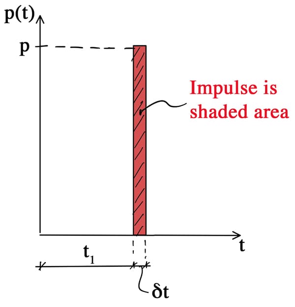
Fig 1. Impulse associated with the force $p(t)$ applied for duration $\delta t$ .

Now, let's think about applying an impulse to a SDoF system. We'll see below that we can determine an expression for the resulting free vibration response of the system. Remember, the impulse is a very short duration, high magnitude load. So, it will induce a short duration driven response followed by a decaying (we'll assume a damped system) free vibration response.

So, how do we use this new information to simulate the response of a SDoF system to general dynamic loading? The trick is to consider the general dynamic loading as a sequence of short duration impulses. Each impulse will induce a free vibration response. To obtain the overall dynamic response, we simply superimpose the free vibration responses due to each impulse, Fig. 2.

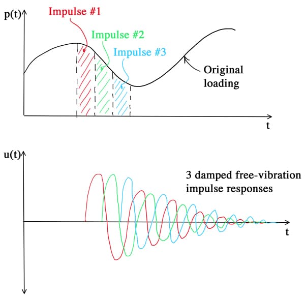
Fig 2. General dynamic loading considered as a sequence of $N$ impulses yielding $N$ free vibration responses that can be superimposed to obtain the response to the original dynamic loading.

Hopefully you can see that at a concept level, there's not much complexity to the Duhamel integral. It's a very simple but versatile tool. There is one limitation to be aware of. Because we rely on superposition to obtain the overall structural response we must assume the behaviour of the dynamic system is linear. If this is not the case, an alternative solution strategy should be sought, such as direct integration of the equation(s) of motion. We cover this in more detail in our Multi-Degree of Freedom Dynamics course.

Damped impulse response

Our next task is to determine an expression for the impulse response of our SDoF system. We start by considering Newton's second law which states that the rate of change of velocity is directly proportional to the force that causes it, mathematically we have,

F(\tau) = m\frac{\mathrm{d}v}{\mathrm{d}\tau} \tag{2}

Rearranging slightly we have,

F(\tau)\mathrm{d}\tau = m \mathrm{d}v \tag{3}

Notice that $F(\tau)\mathrm{d}\tau$ is actually an impulse; recall from above that the impulse associated with force $p(t)$ was the area below the force-time history, $p(t)\delta t$ . We can see that the impulse $F(\tau)\mathrm{d}\tau$ induces an instantaneous change in velocity, $\mathrm{d}v$ . Also note that we've introduced the time variable $\tau$ , distinct from $t$ , to represent the time of application of a specific impulse. This will become clearer when we see both $\tau$ and $t$ in the same expression below.

The instantaneous change in velocity, $\mathrm{d}v$ can equally be interpreted as an initial velocity, $v_0$ associated with the application of the impulse,

\mathrm{d}v = v_0 = \frac{F(\tau)\mathrm{d}\tau}{m} \tag{4}

Now our problem reduces to determining the free vibration response of a SDoF system with non-zero initial velocity $v_0$ at time $\tau$ . We can show that the damped free vibration response of a SDoF system is given by,

u(t) = e^{-\xi\omega_n t}\left[\frac{v_0 + u_0\xi\omega_n}{\omega_d}\sin(\omega_d t) + u_0\cos(\omega_d t)\right] \tag{5}

where, $\xi$ is the damping ratio, $\omega_n$ is the angular natural frequency, $\omega_d$ is the damped natural frequency and $u_0$ is the initial displacement. We cover the derivation of this equation in our Fundamentals of Structural Dynamics course.

Now, if we assume the impulse is applied at time $\tau$ , let $u_0=0$ and let $v_0$ equal to the value in equation 4, we can obtain an expression for the incremental response, $\mathrm{d}u(t)$ due to the impulse $F(\tau)\mathrm{d}\tau$ applied at time $\tau$ ,

\tag{6} \mathrm{d}u(t) = e^{-\xi\omega_n(t-\tau)}\left[\frac{F(\tau)\mathrm{d}\tau}{m\omega_d}\sin\omega_d(t-\tau)\right]

Note that we now have the quantity of time elapsed since the impulse was applied, denoted as $t-\tau$ . This is why we introduced the time variable $\tau$ originally. We're not quite finished; remember that to get the total response of the system at time $t$ , we need to sum up or superimpose the influence of all of the impulses applied, up to this point in time. We can do this by integrating both sides of equation 6,

\boxed{u(t) = \frac{1}{m\omega_d}\int_0^t F(\tau) e^{-\xi\omega_n(t-\tau)}\sin \omega_d (t-\tau)\mathrm{d}\tau} \tag{7}

This expression is what we refer to as Duhamel's integral - the next step is to solve it.

Next Lesson

2. Analytical Solution